The goal of the package is to provide a flexible method of applying stability selection (Meinshausen and Buhlmann, 2010) with various model types, and the framework for triangulating the results for multiple models (Lima et al., 2021).
stabilise() performs stability selection on a range of
models to identify variables truly associated with an outcome.triangulate() identifies which variables are most
likely to be associated with an outcome across all models.stab_plot() allows visualisation of either
stabilise() or triangulate() outputs.simulate_data() allows the simulation of datasets to
facilitate user the comparison of various statistical methods.You can install this package from CRAN as follows:
install.packages("stabiliser")Or using the developmental version as follows:
devtools::install_github("roberthyde/stabiliser")The stabiliser_example is a simulated example dataset with 50 observations of the following variables:
yy:
causal1, causal2…y:
junk1, junk2…library(stabiliser)
data("stabiliser_example")stabilise()To attempt to identify which variables are truly “causal” in this
dataset using a selection stability approach, use the
stabilise() function as follows:
stable_enet <- stabilise(data = stabiliser_example,
                         outcome = "y")
Access the stability (percentage of bootstrap resamples where a given variable was selected by a given model) results for elastic net as follows:
stable_enet$enet$stability
#> # A tibble: 100 x 7
#>    variable mean_coefficient ci_lower ci_upper bootstrap_p stability stable
#>    <chr>               <dbl>    <dbl>    <dbl>       <dbl>     <dbl> <chr>
#>  1 causal1              2.58   0.207    5.45             0      90   *
#>  2 causal3              2.59   0.222    6.49             0      78.5 *
#>  3 causal2              2.12   0.0803   5.01             0      78   *
#>  4 junk14               2.58   0.0695   7.31             0      71   <NA>
#>  5 junk45               2.54   0.0526   5.76             0      63.5 <NA>
#>  6 junk13               2.55   0.136    6.07             0      60.5 <NA>
#>  7 junk88               1.88   0.0300   4.87             0      58   <NA>
#>  8 junk86               1.59   0.110    4.98             0      57   <NA>
#>  9 junk90               1.98   0.161    5.20             0      56   <NA>
#> 10 junk65              -1.25  -3.65    -0.0244           0      46.5 <NA>
#> # ... with 90 more rows
This ranks the variables by stability, and displays the mean coefficients, 95% confidence interval and bootstrap p-value. It also displays whether the variable is deemed “stable”, in this case 3 out of the 4 truly causal variables are identified as “stable”, with no false positives.
By default, this implements an elastic net algorithm over a number of bootstrap resamples of the dataset (200 resamples for small datasets). The stability of each variable is then calculated as the proportion of bootstrap repeats where that variable is selected in the model.
stabilise() also permutes the outcome several times (10
by default for small datasets) and performs the same process on each
permuted dataset (20 bootstrap resamples for each by default).
This allows a permutation threshold to be calculated. Variables with a non-permuted stability % above this threshold are deemed “stable” as they were selected in a higher proportion of bootstrap resamples than in the permuted datasets, where we know there is no association between variables and the outcome.
The permutation threshold is available as follows:
stable_enet$enet$perm_thresh
#> [1] 74triangulate()Our confidence that a given variable is truly associated with a given outcome might be increased if it is identified in multiple model types.
Specify multiple model types (elastic net, mbic and mcp) for
comparison using the stabilise() function as follows:
stable_combi <- stabilise(data = stabiliser_example,
                         outcome = "y",
                         models = c("enet",
                                    "mbic",
                                    "mcp"))
The stability of variables is available for all model types as before.
The stability results from these three models stored within
stable_combi can be combined using triangulate
as follows:
triangulated <- triangulate(stable_combi)
triangulated
#> $combi
#> $combi$stability
#> # A tibble: 100 x 4
#>    variable stability bootstrap_p stable
#>    <chr>        <dbl>       <dbl> <chr>
#>  1 causal1       62.3     0.00292 *
#>  2 causal2       46.5     0       *
#>  3 causal3       45.3     0       *
#>  4 junk13        38       0       <NA>
#>  5 junk14        37.8     0       <NA>
#>  6 junk88        34.5     0       <NA>
#>  7 junk45        29.5     0       <NA>
#>  8 junk90        28.8     0       <NA>
#>  9 junk86        28       0.0204  <NA>
#> 10 junk65        19.8     0       <NA>
#> # ... with 90 more rows
#>
#> $combi$perm_thresh
#> [1] 43
This shows variables consistently being identified as being stable across multiple model types, and consequently increasing our confidence that they are truly associated with the outcome.
Triangulating the results for stability selection across multiple
model types generally provides better performance at identifying truly
causal variables than single model approaches (Lima et al., 2021). As
shown in this example, the triangulated approach identifies 3 out of the
4 truly causal variables as being “stable”, and being highly likely to
be associated with the outcome y.
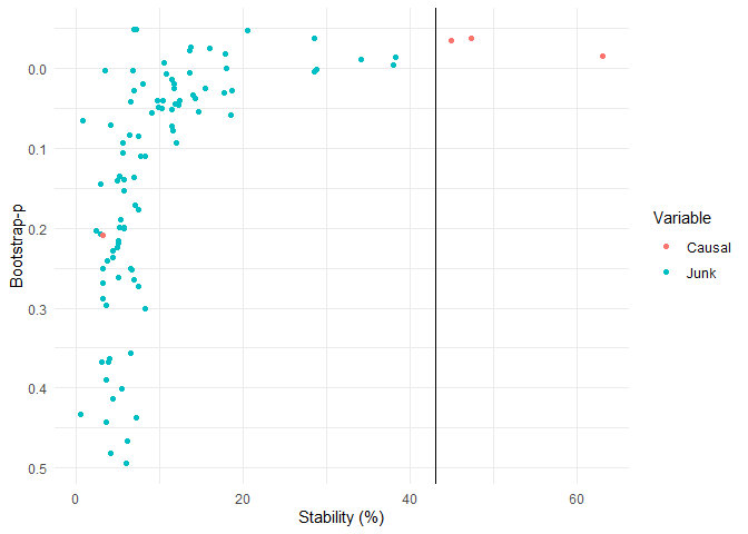
stab_plot()Both stabilise() and triangulate() outputs
can be plotted using stab_plot() as follows, with causal
and junk variables highlighted for this example:
stab_plot(stabiliser_object = triangulated)
simulate_data()To determine the optimum statistical approach, it can be useful to simulate datasets that are simular to those being explored within a research project, but with known outcomes.
The package includes a simulate_data() function, which
allows the user to simulate a dataset as follows:
nrows: the number of rows to simulate.ncols: The number of columns to simulate.n_true: The number of variables truly associated with
the outcome.amplitude: The strength of association between true
variables and the outcome.For example, simulating a 5 row dataset, with 5 explanatory variables, where 2 variables are truly associated with the outcome with a signal strength of 8 would be conducted using the code below. Note that the variables simulated to be truly associated with the outcome are labeled as “true_”, and variables that are randomly generated labeled as “junk_”.
simulate_data(nrows=5,
              ncols=5,
              n_true=2,
              amplitude=8)
#>     outcome    junk_V1    true_V2    true_V3    junk_V4     junk_V5
#> 1  0.221365 -1.4714379  0.1265166 -0.2050986 -1.9603030  0.74586529
#> 2 -4.524082  0.8873447 -0.6569296 -0.4972537  1.0603469  1.03974907
#> 3 -3.948917  0.4930688 -0.4016229 -0.7191238 -0.7291698 -0.79151647
#> 4 -2.617451 -0.2217698 -0.6222874 -0.1586967  0.9645390 -0.03753633
#> 5  4.613613  0.1590784 -0.3425437  1.6222826  1.4840578  0.15464136
It can also be interesting to simulate datasets with no variables
associated with the outcome (other than by chance). This can be done by
setting n_true to zero (or leaving to the default of
zero).
simulate_data(nrows=5,
              ncols=5,
              n_true=0)
#>      outcome    junk_V1     junk_V2    junk_V3     junk_V4     junk_V5
#> 1  2.2007843 -0.8401319 -1.52055028 -1.1568187  1.94737237 -0.12843586
#> 2 -0.1496611  0.7128174  0.50553131  0.8950869  0.02989857 -0.51574352
#> 3 -0.9676750  1.2115235  0.88489231  0.6895640 -0.39529438 -0.16517106
#> 4  0.3468111  1.3880437 -0.31587319  1.2727221  0.29985638  0.06233299
#> 5 -0.9533052 -1.0614021  0.09315892 -0.4079483 -0.17326474 -0.98466363
By using simulated datasets with no signal other than by chance, it is possible to explore various modeling approaches to determine how many false positive variables might be selected with a given approach.
Lima, E., Hyde, R., Green, M., 2021. Model selection for inferential models with high dimensional data: synthesis and graphical representation of multiple techniques. Sci. Rep. 11, 412. https://doi.org/10.1038/s41598-020-79317-8
Meinshausen, N., Buhlmann, P., 2010. Stability selection. J. R. Stat. Soc. Ser. B (Statistical Methodol. 72, 417–473. https://doi.org/10.1111/j.1467-9868.2010.00740.x