![]()
![]()
The goal of {simodels} is to provide a simple, tidy, and flexible framework for developing spatial interaction models (SIMs). SIMs estimate the amount of movement between spatial entities and can be used for many things, including to support evidence-based investment in sustainable transport infrastructure and prioritisation of location options for public services.
Unlike many software tools designed to support spatial interaction modelling, {simodels} does not define (or even encourage use of) any particular functional forms or modelling frameworks for predicting movement between origins and destinations. Instead, it provides a framework enabling you to use model function forms or models of your choosing, ensuring flexibility and encouraging flexibility.
Install the package as follows:
install.packages("remotes") # if not already installedremotes::install_github("robinlovelace/simodels")To get the develoment version do:
devtools::load_all()Run a basic SIM as follows:
library(simodels)
library(dplyr)
# prepare OD data
od = si_to_od(
  origins = si_zones,        # origin locations
  destinations = si_zones,   # destination locations
  max_dist = 5000            # maximum distance between OD pairs
  )
# specify a function
gravity_model = function(beta, d, m, n) {
  m * n * exp(-beta * d / 1000)
}
# perform SIM
od_res = si_calculate(
  od,
  fun = gravity_model,
  d = distance_euclidean,
  m = origin_all,
  n = destination_all,
  constraint_production = origin_all,
  beta = 0.9
  )
# visualize the results
plot(od_res$distance_euclidean, od_res$interaction)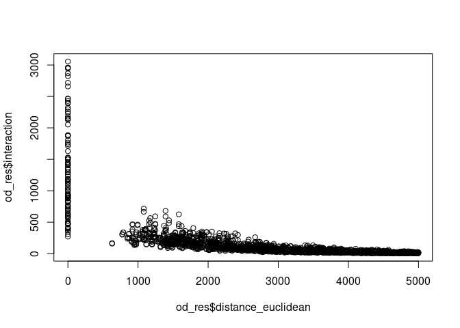
What just happened? We created an ‘OD data frame’ with the function
si_to_od() from geographic origins and destinations, and
then estimated a simple ‘production constrained’ (with the
constraint_production argument) gravity model based on the
population in origin and destination zones and a custom distance decay
function with si_calculate(). As the example above shows,
the package allows/encourages you to define and use your own functions
to estimate the amount of interaction/movement between places.
The approach is also ‘tidy’, allowing use of {simodels} functions in {dplyr} pipelines:
od_res = od %>%
  si_calculate(fun = gravity_model,
               m = origin_all,
               n = destination_all,
               d = distance_euclidean,
               constraint_production = origin_all,
               beta = 0.3)
od_res %>%
  select(interaction)
Simple feature collection with 2505 features and 1 field
Geometry type: LINESTRING
Dimension: XY
Bounding box: xmin: -1.743949 ymin: 53.71552 xmax: -1.337493 ymax: 53.92906
Geodetic CRS: WGS 84
# A tibble: 2,505 × 2
interaction geometry
<dbl> <LINESTRING [°]>
1 2177. (-1.400108 53.92906, -1.400108 53.92906)
2 632. (-1.400108 53.92906, -1.346497 53.92305)
3 556. (-1.346497 53.92305, -1.400108 53.92906)
4 1382. (-1.346497 53.92305, -1.346497 53.92305)
5 449. (-1.346497 53.92305, -1.357667 53.88306)
6 794. (-1.704658 53.91073, -1.704658 53.91073)
7 749. (-1.704658 53.91073, -1.6876 53.90066)
8 287. (-1.704658 53.91073, -1.743949 53.88035)
9 267. (-1.704658 53.91073, -1.710657 53.87087)
10 186. (-1.704658 53.91073, -1.694076 53.86729)
# ℹ 2,495 more rowsThe resulting estimates of interaction, returned in the column
interaction and plotted with distance in the graphic above,
resulted from our choice of spatial interaction model inputs, allowing a
wide range of alternative approaches to be implemented. This flexibility
is a key aspect of the package, enabling small and easily modified
functions to be implemented and tested.
The output of si_calculate() is a geographic object that
can be plotted with sf’s plot method (or other geographic
data visualisation packages):
plot(od_res["interaction"], logz = TRUE)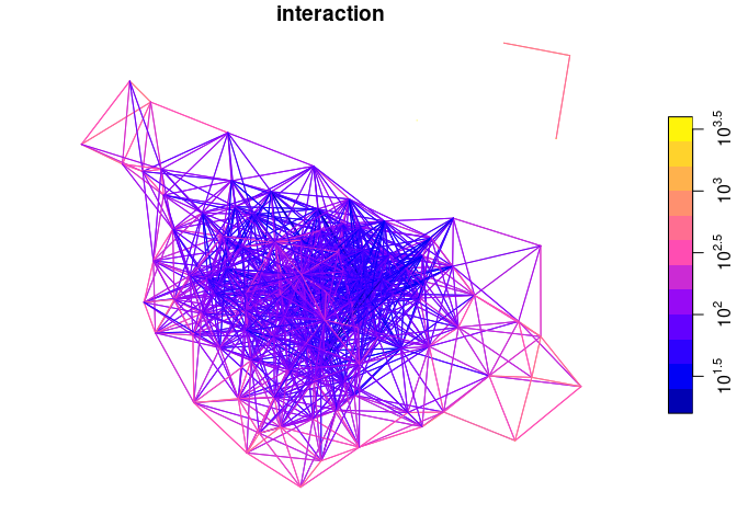
The si_to_od() function transforms geographic entities
(typically polygons and points) into a data frame representing the full
combination of origin-destination pairs that are less than
max_dist meters apart. A common saying in data science is
that 80% of the effort goes into the pre-processing stage. This is
equally true for spatial interaction modelling as it is for other types
of data intensive analysis/modelling work. So what does this function
return?
The function allows you to use any variable in the origin or
destination data by joining all attributes onto the OD data frame, with
column names appended with origin and
destination.
The approach works equally well for ‘bipartite’ SIMs, in which origin and destination points are different (Hasova et al. 2022). The following example implements a bipartite SIM that estimates the number of trips from administrative zones to pubs in Leeds:
# Set n. trips to pubs, assuming that for every trip to the pub there are
# 50 trips to work (this would be validated/tested/modelled in empirical work)
zones_pubs = si_zones %>%
  mutate(to_pubs = all / 50)
pubs_example = si_pubs %>%
  filter(grepl(pattern = "Chemic|Nag", x = name))
pubs_example$size = c(100, 80)
od_to_pubs = si_to_od(zones_pubs, pubs_example)
od_to_pubs_result = od_to_pubs %>%
  si_calculate(fun = gravity_model,
               m = origin_to_pubs,
               n = destination_size,
               d = distance_euclidean,
               beta = 0.5,
               constraint_production = origin_to_pubs)
od_to_pubs_result %>%
  select(O, D, destination_name, interaction)
Simple feature collection with 214 features and 4 fields
Geometry type: LINESTRING
Dimension: XY
Bounding box: xmin: -1.743949 ymin: 53.71552 xmax: -1.337493 ymax: 53.92906
Geodetic CRS: WGS 84
# A tibble: 214 × 5
O D destination_name interaction geometry
<chr> <chr> <chr> <dbl> <LINESTRING [°]>
1 E02002330 127960333 The Chemic Tavern 18.4 (-1.400108 53.92906, -1.55…
2 E02002331 127960333 The Chemic Tavern 15.9 (-1.346497 53.92305, -1.55…
3 E02002332 127960333 The Chemic Tavern 25.5 (-1.704658 53.91073, -1.55…
4 E02002333 127960333 The Chemic Tavern 38.7 (-1.6876 53.90066, -1.5528…
5 E02002334 127960333 The Chemic Tavern 20.9 (-1.357667 53.88306, -1.55…
6 E02002335 127960333 The Chemic Tavern 19.9 (-1.470966 53.89184, -1.55…
7 E02002336 127960333 The Chemic Tavern 25.5 (-1.624775 53.88589, -1.55…
8 E02002337 127960333 The Chemic Tavern 37.2 (-1.743949 53.88035, -1.55…
9 E02002338 127960333 The Chemic Tavern 36.8 (-1.710657 53.87087, -1.55…
10 E02002339 127960333 The Chemic Tavern 29.0 (-1.694076 53.86729, -1.55…
# ℹ 204 more rowsWe can plot the top 20 desire lines between zone centroids and the 2 pubs in the example dataset as follows:
library(tmap)
tmap_mode("view")
od_to_pubs_result %>%
  top_n(n = 50, wt = interaction) %>%
  tm_shape() +
  tm_lines(col = "interaction", palette = "viridis", scale = 2)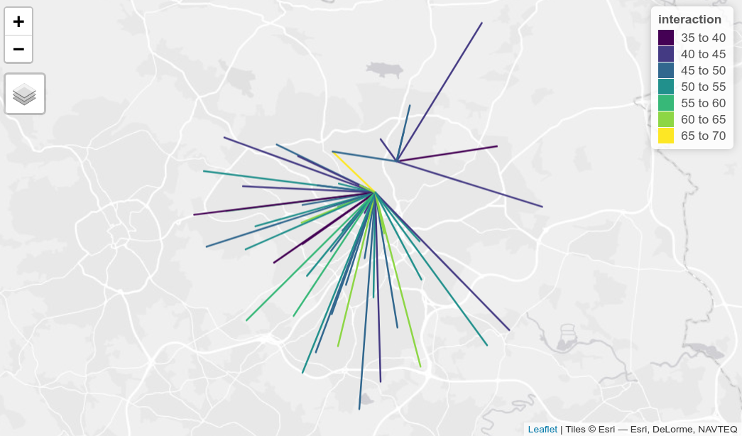
We would be interested to hear how the approach presented in this package compared with other implementations such as those presented in the links below. If anyone would like to try the approach or implement it in another language feel free to get in touch via the issue tracker.
For details on what SIMs are and how they have been defined
mathematically and in code from first principles, see the sims
vignette.
To dive straight into using {simodels} to develop SIMs, see the Get started vignette.
For a detailed introduction to SIMs, support by reproducible R code, see Adam Dennett’s 2018 paper.
spflow R
packagespint Python
packagegravity
R packagemobility
R package