![]()
![]()
simMetric is an R package that provides metrics (and
their Monte Carlo standard errors) for the assessment of statistical
methods in simulation studies. This package includes metrics that are
calculated as per this tutorial published by Tim
Morris, Ian White and Michael Crowther. For an in-depth description on
the calculation and interpretation, and how to perform a simulation
study in general, refer to the tutorial.
You can install the development version of simMetric from GitHub with:
# install.packages("remotes")
remotes::install_github("RWParsons/simMetric")
Or install from CRAN
install.packages("simMetric")
Here is a basic example that performs a simulation study, evaluates the metrics and plots the results:
library(simMetric)
library(tidyverse)data_generator <- function(n_obs, noise = 1, effect = 0, s = 42) {
set.seed(s)
x <- rnorm(n = n_obs, mean = 0, sd = 1)
y <- x * effect + rnorm(n = n_obs, mean = 0, sd = noise)
data.frame(x = x, y = y)
}
assess_lm <- function(data) {
model <- lm(y ~ x, data = data)
model %>%
broom::tidy(., conf.int = T) %>%
filter(term == "x") %>%
select(-any_of(c("term", "statistic"))) %>%
add_column(model = "with_intercept")
}
assess_lm_no_intercept <- function(data) {
model <- lm(y ~ 0 + x, data = data)
model %>%
broom::tidy(., conf.int = T) %>%
filter(term == "x") %>%
select(-any_of(c("term", "statistic"))) %>%
add_column(model = "without_intercept")
}
assess_lm(data_generator(n_obs = 10, noise = 0.1, effect = 1))
#> # A tibble: 1 × 6
#> estimate std.error p.value conf.low conf.high model
#> <dbl> <dbl> <dbl> <dbl> <dbl> <chr>
#> 1 0.927 0.0640 0.000000504 0.779 1.07 with_intercept
assess_lm_no_intercept(data_generator(n_obs = 10, noise = 0.1, effect = 1))
#> # A tibble: 1 × 6
#> estimate std.error p.value conf.low conf.high model
#> <dbl> <dbl> <dbl> <dbl> <dbl> <chr>
#> 1 0.941 0.0501 0.0000000158 0.828 1.05 without_interceptThe number of unique seeds represents the number of
simulations to be done (100 in this example)
g <- expand.grid(
  seed = 1:100,
  n_obs = seq(from = 10, to = 50, by = 10),
  noise = 0.1,
  effect = 0.5
)Since we want to simulate the multiple models, and we want to apply
the same datasets to each set of models, we have one row returned per
model that we are simulating. This way, fit_one_model is
run once per simulated dataset, and the generated data is used for all
included models.
fit_one_model <- function(grid, row) {
  inputs <- grid[row, ]
  d <- data_generator(
    n_obs = inputs$n_obs,
    noise = inputs$noise,
    effect = inputs$effect,
    s = inputs$seed
  )

  cbind(
    rbind(assess_lm(d), assess_lm_no_intercept(d)),
    inputs
  )
}fit_one_model(g, 1)
#> Warning in data.frame(..., check.names = FALSE): row names were found from a
#> short variable and have been discarded
#> estimate std.error p.value conf.low conf.high model seed
#> 1 0.4483862 0.04487337 8.537408e-06 0.3449081 0.5518644 with_intercept 1
#> 2 0.4557942 0.04388530 2.608370e-06 0.3565188 0.5550697 without_intercept 1
#> n_obs noise effect
#> 1 10 0.1 0.5
#> 2 10 0.1 0.5data.frame.library(parallel)
cl <- parallelly::autoStopCluster(makeCluster(detectCores()))
clusterExport(cl, ls()[!ls() %in% "cl"]) # send the grid and functions to each node
x <- clusterEvalQ(cl, require(tidyverse, quietly = T)) # load the tidyverse on each node
start <- Sys.time()
ll <- parLapply(
cl,
1:nrow(g),
function(r) fit_one_model(grid = g, r)
)
par_res <- do.call("rbind", ll)
head(par_res)
#> estimate std.error p.value conf.low conf.high model seed
#> 1 0.4483862 0.04487337 8.537408e-06 0.3449081 0.5518644 with_intercept 1
#> 2 0.4557942 0.04388530 2.608370e-06 0.3565188 0.5550697 without_intercept 1
#> 3 0.5239730 0.04153620 1.463669e-06 0.4281904 0.6197557 with_intercept 2
#> 4 0.5269444 0.03844832 2.464367e-07 0.4399683 0.6139206 without_intercept 2
#> 5 0.4758010 0.02818650 1.537607e-07 0.4108028 0.5407992 with_intercept 3
#> 6 0.4786038 0.02884696 4.686118e-08 0.4133474 0.5438601 without_intercept 3
#> n_obs noise effect
#> 1 10 0.1 0.5
#> 2 10 0.1 0.5
#> 3 10 0.1 0.5
#> 4 10 0.1 0.5
#> 5 10 0.1 0.5
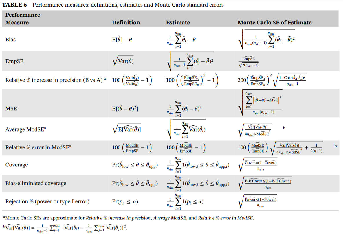
#> 6 10 0.1 0.5{simMetric}simMetric::join_metrics()df_metrics <- join_metrics(
par_res,
id_cols = c("n_obs", "model"),
metrics = c("coverage", "mse", "modSE", "empSE", "relativeErrorModSE"),
ll_col = "conf.low",
ul_col = "conf.high",
true_value = "effect",
estimates_col = "estimate",
se_col = "std.error"
)
head(df_metrics)
#> # A tibble: 6 × 12
#> n_obs model cover…¹ cover…² mse mse_m…³ modSE modSE…⁴ empSE empSE…⁵
#> <dbl> <chr> <dbl> <dbl> <dbl> <dbl> <dbl> <dbl> <dbl> <dbl>
#> 1 10 with_inte… 0.97 0.0171 1.21e-3 1.93e-4 0.0370 1.55e-3 0.0349 0.00248
#> 2 10 without_i… 0.99 0.00995 9.88e-4 1.58e-4 0.0347 1.46e-3 0.0315 0.00224
#> 3 20 with_inte… 0.94 0.0237 6.13e-4 1.14e-4 0.0248 7.44e-4 0.0249 0.00177
#> 4 20 without_i… 0.92 0.0271 6.08e-4 1.13e-4 0.0241 7.35e-4 0.0248 0.00176
#> 5 30 with_inte… 0.95 0.0218 4.92e-4 6.65e-5 0.0193 4.08e-4 0.0223 0.00158
#> 6 30 without_i… 0.92 0.0271 4.61e-4 6.55e-5 0.0189 3.78e-4 0.0216 0.00153
#> # … with 2 more variables: relativeErrorModSE <dbl>,
#> # relativeErrorModSE_mcse <dbl>, and abbreviated variable names ¹coverage,
#> # ²coverage_mcse, ³mse_mcse, ⁴modSE_mcse, ⁵empSE_mcsegroup_by() and
summarise()df_metrics <-
par_res %>%
group_by(n_obs, model) %>%
summarise(
coverage_estimate = coverage(true_value = effect, ll = conf.low, ul = conf.high, get = "coverage"),
coverage_mcse = coverage(true_value = effect, ll = conf.low, ul = conf.high, get = "coverage_mcse"),
mean_squared_error_estimate = mse(true_value = effect, estimates = estimate, get = "mse"),
mean_squared_error_mcse = mse(true_value = effect, estimates = estimate, get = "mse_mcse")
)
#> `summarise()` has grouped output by 'n_obs'. You can override using the
#> `.groups` argument.
head(df_metrics)
#> # A tibble: 6 × 6
#> # Groups: n_obs [3]
#> n_obs model coverage_estimate coverage_mcse mean_squared…¹ mean_…²
#> <dbl> <chr> <dbl> <dbl> <dbl> <dbl>
#> 1 10 with_intercept 0.97 0.0171 0.00121 1.93e-4
#> 2 10 without_intercept 0.99 0.00995 0.000988 1.58e-4
#> 3 20 with_intercept 0.94 0.0237 0.000613 1.14e-4
#> 4 20 without_intercept 0.92 0.0271 0.000608 1.13e-4
#> 5 30 with_intercept 0.95 0.0218 0.000492 6.65e-5
#> 6 30 without_intercept 0.92 0.0271 0.000461 6.55e-5
#> # … with abbreviated variable names ¹mean_squared_error_estimate,
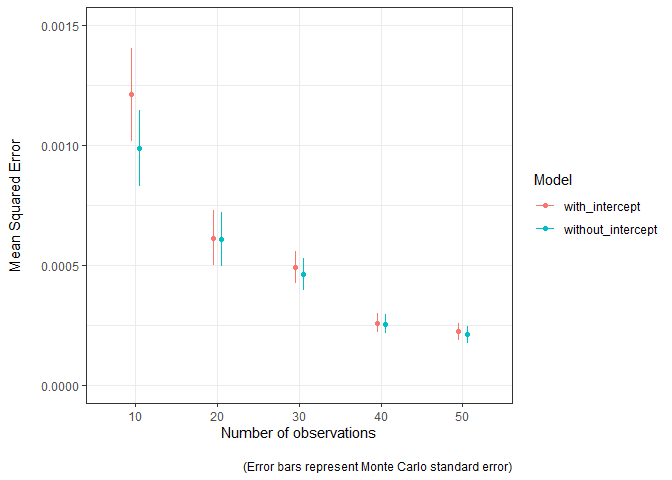
#> # ²mean_squared_error_mcseThe model estimates are closer to the truth (MSE is lower) as the sample used to fit the model increases in size. The Monte Carlo standard error can easily be visualised to convey the uncertainty in these estimates. The model without the intercept term seems to be a bit better, mostly when sample sizes are lower.
df_metrics %>%
  ggplot(aes(as.factor(n_obs), mean_squared_error_estimate, group = model, colour = model)) +
  geom_point(position = position_dodge(width = 0.2)) +
  geom_errorbar(aes(
    ymin = mean_squared_error_estimate - mean_squared_error_mcse,
    ymax = mean_squared_error_estimate + mean_squared_error_mcse
  ),
  width = 0, position = position_dodge(width = 0.2)
  ) +
  theme_bw() +
  labs(
    x = "Number of observations",
    y = "Mean Squared Error\n",
    colour = "Model",
    caption = "\n(Error bars represent Monte Carlo standard error)"
  ) +
  scale_y_continuous(labels = scales::comma, limits = c(0, 0.0015))