![]()
![]()
![]()
The goal of sgo is to provide a set of methods to
transform ETRS89 coordinates to the equivalent OSGB36 National Grid
coordinates, and vice-versa, using the Ordnance
Survey’s National Grid Transformation Model OSTN15. Additionally, it
also has the ability to calculate distances and areas from groups of
points defined in any of the coordinate systems supported.
The Coordinate Systems supported by sgo are:
Please note that this package assumes that the Coordinate Reference Systems (CRS) ETRS89 and WGS84 are the same within the UK, but this shouldn’t be a problem for most civilian use of GPS satellites. If a high-precision transformation between WGS84 and ETRS89 is required then it is recommended to use a different package to do the conversion.
According to the Transformations and OSGM15 User Guide, p. 8: “…ETRS89 is a precise version of the better known WGS84 system optimised for use in Europe; however, for most purposes it can be considered equivalent to WGS84.” and “For all navigation, mapping, GIS, and engineering applications within the tectonically stable parts of Europe (including UK and Ireland), the term ETRS89 should be taken as synonymous with WGS84.”.
You can install the released version of sgo from CRAN with:
install.packages("sgo")And the development version from GitHub with:
# install.packages("remotes")
remotes::install_github("clozanoruiz/sgo")library(sgo)
## sgo_points creation (from lists, matrices or dataframes)
sr <- sgo_points(list(-3.9369, 56.1165), epsg=4326)
sr
#> An sgo object with 1 feature (point)
#> dimension: XY
#> EPSG: 4326
#> x y
#> 1 -3.9369 56.1165
ln <- c(-4.22472, -2.09908)
lt <- c(57.47777, 57.14965)
n <- c("Inverness", "Aberdeen")
df <- data.frame(n, ln, lt, stringsAsFactors = FALSE)
locs <- sgo_points(df, coords=c("ln", "lt"), epsg=4326)
library(maps)
map('world', regions=('uk'), xlim=c(-9, 0), ylim=c(54.5, 60.9))
points(x=sr$x, y=sr$y, pch=0, col="green")
points(locs, pch=0, col="red")
text(locs, labels=locs$n, pos=1, cex=0.9)
text(sr, labels="Stirling", pos=1, cex=0.9)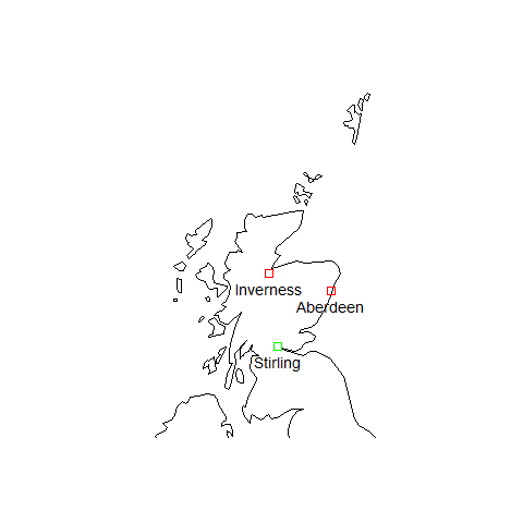
## Convert coordinates to OS National Grid reference
bv <- sgo_points(list(x=247455, y=706338, name="Ben Venue"),
coords=c("x", "y"), epsg=27700)
sgo_bng_ngr(bv)$ngr
#> [1] "NN 47455 06338"
# notice the truncating:
sgo_bng_ngr(bv, digits=8)$ngr
#> [1] "NN 4745 0633"


## Convert from lon/lat to BNG
lon <- c(-4.25181,-3.18827)
lat <- c(55.86424, 55.95325)
pts <- sgo_points(list(longitude=lon, latitude=lat), epsg=4326)
sgo_lonlat_bng(pts)
#> An sgo object with 2 features (points)
#> dimension: XY
#> EPSG:      27700
#>          x        y
#> 1 259174.4 665744.8
#> 2 325899.1 673996.1


## sgo_transform is a wrapper for all the conversions available.

# to BNG:
sgo_transform(locs, to=27700)
#> An sgo object with 2 features (points) and 1 field
#> dimension: XY
#> EPSG:      27700
#>          x        y         n
#> 1 266698.8 845243.9 Inverness
#> 2 394104.5 806535.9  Aberdeen

# to OSGB36 (historical):
sgo_transform(locs, to=4277)
#> An sgo object with 2 features (points) and 1 field
#> dimension: XY
#> EPSG:      4277
#>           x        y         n
#> 1 -4.223366 57.47804 Inverness
#> 2 -2.097450 57.14985  Aberdeen

# to Pseudo-Mercator:
sgo_transform(locs, to=3857)
#> An sgo object with 2 features (points) and 1 field
#> dimension: XY
#> EPSG:      3857
#>           x       y         n
#> 1 -470293.7 7858404 Inverness
#> 2 -233668.5 7790768  Aberdeen


## Convert OS National Grid references to ETRS89
munros <- data.frame(
  ngr=c("NN 1652471183", "NN 98713 98880",
         "NN9521499879", "NN96214 97180"),
  name=c("Beinn Nibheis", "Beinn Macduibh",
          "Am Bràigh Riabhach", "Càrn an t-Sabhail"))
sgo_transform(sgo_ngr_bng(munros, col="ngr"), to=4258)
#> An sgo object with 4 features (points) and 1 field
#> dimension: XY
#> EPSG:      4258
#>           x        y               name
#> 1 -5.005929 56.79589      Beinn Nibheis
#> 2 -3.672139 57.06976     Beinn Macduibh
#> 3 -3.730236 57.07795 Am Bràigh Riabhach
#> 4 -3.712631 57.05394  Càrn an t-Sabhail


## Calculate distances
# Distance in metres from one point to 2 other points
p1 <- sgo_points(list(-3.9369, 56.1165), epsg=4326)
lon <- c(-4.25181,-3.18827)
lat <- c(55.86424, 55.95325)
pts <- sgo_points(list(longitude=lon, latitude=lat), epsg=4326)
p1.to.pts <- sgo_distance(p1, pts, by.element = TRUE)
p1.to.pts
#> [1] 34279.98 50081.63

# Perimeter in metres of a polygon defined as a series of ordered points:
lon <- c(-6.43698696, -6.43166843, -6.42706831, -6.42102546,
-6.42248238, -6.42639092, -6.42998435, -6.43321409)
lat <- c(58.21740316, 58.21930597, 58.22014035, 58.22034112,
58.21849188, 58.21853606, 58.21824033, 58.21748949)
pol <- sgo_points(list(lon, lat), epsg=4326)
# Let's create a copy of the polygon with its coordinates shifted one position
# so that we can calculate easily the distance between vertices
coords <- sgo_coordinates(pol)
pol.shift.one <- sgo_points(rbind(coords[-1, ], coords[1, ]), epsg=pol$epsg)
perimeter <- sum(sgo_distance(pol, pol.shift.one, by.element=TRUE))
perimeter
#> [1] 2115.33


## Area of an ordered set of points
A <- sgo_area(pol)
sprintf("%1.2f", A)
#> [1] "133610.63"
# Interpolate new vertices (here every 10 metres) if more accuracy is needed
A <- sgo_area(pol, interpolate=10)
sprintf("%1.2f", A)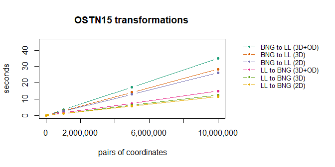
#> [1] "133610.64"Very simple benchmark in a Intel(R) Core(TM) i7-6700HQ CPU @2.60GHz, and 16 GB of RAM. See the code of this README file to see the R statements used.