![]()
The goal of reportRmd is to automate the reporting of clinical data in Rmarkdown environments. Functions include table one-style summary statistics, compilation of multiple univariate models, tidy output of multivariable models and side by side comparisons of univariate and multivariable models. Plotting functions include customisable survival curves, forest plots, and automated bivariate plots.
Installing from CRAN:
install.packages('reportRmd')You can install the development version of reportRmd from GitHub with:
# install.packages("devtools")
devtools::install_github("biostatsPMH/reportRmd", ref="development")rm_compactsumreplace_plot_labelslibrary(reportRmd)
data("pembrolizumab")
rm_covsum(data=pembrolizumab, maincov = 'sex',
covs=c('age','pdl1','change_ctdna_group'),
show.tests=TRUE)| Full Sample (n=94) | Female (n=58) | Male (n=36) | p-value | StatTest | |
|---|---|---|---|---|---|
| age | 0.30 | Wilcoxon Rank Sum | |||
| Mean (sd) | 57.9 (12.8) | 56.9 (12.6) | 59.3 (13.1) | ||
| Median (Min,Max) | 59.1 (21.1, 81.8) | 56.6 (34.1, 78.2) | 61.2 (21.1, 81.8) | ||
| pdl1 | 0.76 | Wilcoxon Rank Sum | |||
| Mean (sd) | 13.9 (29.2) | 15.0 (30.5) | 12.1 (27.3) | ||
| Median (Min,Max) | 0 (0, 100) | 0.5 (0.0, 100.0) | 0 (0, 100) | ||
| Missing | 1 | 0 | 1 | ||
| change ctdna group | 0.84 | Chi Sq | |||
| Decrease from baseline | 33 (45) | 19 (48) | 14 (42) | ||
| Increase from baseline | 40 (55) | 21 (52) | 19 (58) | ||
| Missing | 21 | 18 | 3 |
pembrolizumab |> rm_compactsum( grp = 'sex',
xvars=c('age','pdl1','change_ctdna_group'))| Full Sample (n=94) | Female (n=58) | Male (n=36) | p-value | Missing | |
|---|---|---|---|---|---|
| age | 59.1 (49.5-68.7) | 56.6 (45.8-67.8) | 61.2 (52.0-69.4) | 0.30 | 0 |
| pdl1 | 0.0 (0.0-10.0) | 0.5 (0.0-13.8) | 0.0 (0.0-4.5) | 0.76 | 1 |
| change ctdna group - Increase from baseline | 40 (55%) | 21 (52%) | 19 (58%) | 0.84 | 21 |
var_names <- data.frame(var=c("age","pdl1","change_ctdna_group"),
                          label=c('Age at study entry',
                                  'PD L1 percent',
                                  'ctDNA change from baseline to cycle 3'))

pembrolizumab <- set_labels(pembrolizumab,var_names)

rm_covsum(data=pembrolizumab, maincov = 'sex',
covs=c('age','pdl1','change_ctdna_group'))| Full Sample (n=94) | Female (n=58) | Male (n=36) | p-value | |
|---|---|---|---|---|
| Age at study entry | 0.30 | |||
| Mean (sd) | 57.9 (12.8) | 56.9 (12.6) | 59.3 (13.1) | |
| Median (Min,Max) | 59.1 (21.1, 81.8) | 56.6 (34.1, 78.2) | 61.2 (21.1, 81.8) | |
| PD L1 percent | 0.76 | |||
| Mean (sd) | 13.9 (29.2) | 15.0 (30.5) | 12.1 (27.3) | |
| Median (Min,Max) | 0 (0, 100) | 0.5 (0.0, 100.0) | 0 (0, 100) | |
| Missing | 1 | 0 | 1 | |
| ctDNA change from baseline to cycle 3 | 0.84 | |||
| Decrease from baseline | 33 (45) | 19 (48) | 14 (42) | |
| Increase from baseline | 40 (55) | 21 (52) | 19 (58) | |
| Missing | 21 | 18 | 3 |
rm_uvsum(data=pembrolizumab, response='orr',
covs=c('age','pdl1','change_ctdna_group'))
#> Waiting for profiling to be done...
#> Waiting for profiling to be done...
#> Waiting for profiling to be done...| OR(95%CI) | p-value | N | Event | |
|---|---|---|---|---|
| Age at study entry | 0.96 (0.91, 1.00) | 0.089 | 94 | 78 |
| PD L1 percent | 0.97 (0.95, 0.98) | <0.001 | 93 | 77 |
| ctDNA change from baseline to cycle 3 | 0.002 | 73 | 58 | |
| Decrease from baseline | Reference | 33 | 19 | |
| Increase from baseline | 28.74 (5.20, 540.18) | 40 | 39 |
glm_fit <- glm(orr~change_ctdna_group+pdl1+cohort,
               family='binomial',
               data = pembrolizumab)
rm_mvsum(glm_fit,showN=T)| OR(95%CI) | p-value | N | Event | |
|---|---|---|---|---|
| ctDNA change from baseline to cycle 3 | 0.009 | 73 | 58 | |
| Decrease from baseline | Reference | 33 | 19 | |
| Increase from baseline | 19.99 (2.08, 191.60) | 40 | 39 | |
| PD L1 percent | 0.97 (0.95, 1.00) | 0.066 | 73 | 58 |
| cohort | 73 | 58 | ||
| A | Reference | 14 | 11 | |
| B | 2.6e+07 (0e+00, Inf) | 1.00 | 11 | 11 |
| C | 4.2e+07 (0e+00, Inf) | 1.00 | 10 | 10 |
| D | 0.07 (4.2e-03, 1.09) | 0.057 | 10 | 3 |
| E | 0.44 (0.04, 5.10) | 0.51 | 28 | 23 |
uvsumTable <- rm_uvsum(data=pembrolizumab, response='orr',
covs=c('age','sex','pdl1','change_ctdna_group'),tableOnly = TRUE)
#> Waiting for profiling to be done...
#> Waiting for profiling to be done...
#> Waiting for profiling to be done...
#> Waiting for profiling to be done...

glm_fit <- glm(orr~change_ctdna_group+pdl1,
               family='binomial',
               data = pembrolizumab)
mvsumTable <- rm_mvsum(glm_fit,tableOnly = TRUE)

rm_uv_mv(uvsumTable,mvsumTable)| Unadjusted OR(95%CI) | p | Adjusted OR(95%CI) | p (adj) | |
|---|---|---|---|---|
| Age at study entry | 0.96 (0.91, 1.00) | 0.089 | ||
| sex | 0.11 | |||
| Female | Reference | |||
| Male | 0.41 (0.13, 1.22) | |||
| PD L1 percent | 0.97 (0.95, 0.98) | <0.001 | 0.98 (0.96, 1.00) | 0.024 |
| ctDNA change from baseline to cycle 3 | 0.002 | 0.004 | ||
| Decrease from baseline | Reference | Reference | ||
| Increase from baseline | 28.74 (5.20, 540.18) | 24.71 (2.87, 212.70) |
Shows events, median survival, survival rates at different times and the log rank test. Does not allow for covariates or strata, just simple tests between groups
 rm_survsum(data=pembrolizumab,time='os_time',status='os_status',
 group="cohort",survtimes=c(12,24),
# group="cohort",survtimes=seq(12,36,12),
# survtimesLbls=seq(1,3,1),
 survtimesLbls=c(1,2),
survtimeunit='yr')| Group | Events/Total | Median (95%CI) | 1yr (95% CI) | 2yr (95% CI) |
|---|---|---|---|---|
| A | 12/16 | 8.30 (4.24, Not Estimable) | 0.38 (0.20, 0.71) | 0.23 (0.09, 0.59) |
| B | 16/18 | 8.82 (4.67, 20.73) | 0.32 (0.16, 0.64) | 0.06 (9.6e-03, 0.42) |
| C | 12/18 | 17.56 (7.95, Not Estimable) | 0.61 (0.42, 0.88) | 0.44 (0.27, 0.74) |
| D | 4/12 | Not Estimable (6.44, Not Estimable) | 0.67 (0.45, 0.99) | 0.67 (0.45, 0.99) |
| E | 20/30 | 14.26 (9.69, Not Estimable) | 0.63 (0.48, 0.83) | 0.34 (0.20, 0.57) |
| Log Rank Test | ChiSq | 11.3 on 4 df | ||
| p-value | 0.023 |
library(survival)
data(pbc)
rm_cifsum(data=pbc,time='time',status='status',group=c('trt','sex'),
eventtimes=c(1825,3650),eventtimeunit='day')
#> 106 observations with missing data were removed.| Strata | Event/Total | 1825day (95% CI) | 3650day (95% CI) |
|---|---|---|---|
| 1, f | 7/137 | 0.04 (0.01, 0.08) | 0.06 (0.03, 0.12) |
| 1, m | 3/21 | 0.10 (0.02, 0.27) | 0.16 (0.03, 0.36) |
| 2, f | 9/139 | 0.05 (0.02, 0.09) | 0.09 (0.04, 0.17) |
| 2, m | 0/15 | 0e+00 (NA, NA) | 0e+00 (NA, NA) |
| Gray’s Test | ChiSq | 3.3 on 3 df | |
| p-value | 0.35 |
ggkmcif2(response = c('os_time','os_status'),
cov='cohort',
data=pembrolizumab)
require(ggplot2)
#> Loading required package: ggplot2
forestplotMV(glm_fit)
#> Warning in forestplotMV(glm_fit): NAs introduced by coercion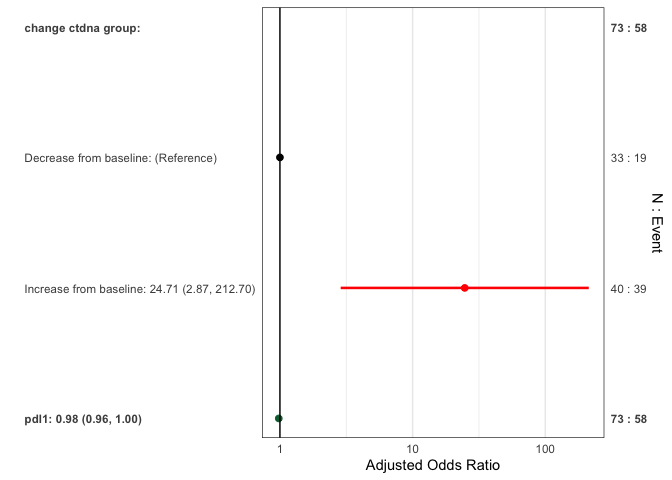
These plots are designed for quick inspection of many variables, not for publication.
require(ggplot2)
plotuv(data=pembrolizumab, response='orr',
covs=c('age','cohort','pdl1','change_ctdna_group'))
#> Boxplots not shown for categories with fewer than 20 observations.
#> Boxplots not shown for categories with fewer than 20 observations.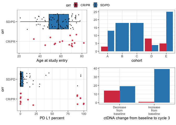
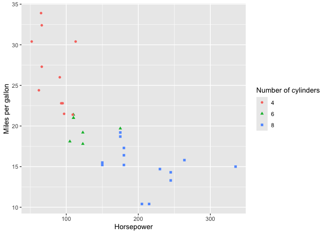
data("mtcars")
mtcars <- mtcars |>
  dplyr::mutate(cyl = as.factor(cyl)) |>
  set_labels(data.frame(var=c("hp","mpg","cyl"),
                        label=c('Horsepower',
                                'Miles per gallon',
                                'Number of cylinders')))
p <- mtcars |>
ggplot(aes(x=hp, y=mpg, color=cyl, shape=cyl)) +
    geom_point()
replace_plot_labels(p)