![]()

![]()


R package of convenience functions to make your workflow faster and
easier. Easily customizable plots (via ggplot2), nice APA
tables exportable to Word (via flextable), easily run
statistical tests or check assumptions, and automatize various other
tasks. Mostly geared at researchers in the psychological sciences. The
package is still under active development. Feel free to open an issue to
ask for help, report a bug, or request a feature.
Top 40 new CRAN packages (2022)!
This is one of the most helpful R packages I’ve used in years! It saves hours of time and patience and is super easy to implement! - Mark (more testimonials)
You can install the rempsyc package directly from
CRAN:
install.packages("rempsyc")Or the development version from the r-universe (note that there is a 24-hour delay with GitHub):
install.packages("rempsyc", repos = c(
  rempsyc = "https://rempsyc.r-universe.dev",
  CRAN = "https://cloud.r-project.org"))
Or from GitHub, for the very latest version:
# If package `remotes` isn't already installed, install it with `install.packages("remotes")`
remotes::install_github("rempsyc/rempsyc")
You can load the package and open the help file, and click “Index” at the bottom. You will see all the available functions listed.
library(rempsyc)
?rempsyc
Dependencies: Because rempsyc is a
package of convenience functions relying on several external packages,
it uses (inspired by the easystats
packages) a minimalist philosophy of only installing packages that you
need when you need them through rlang::check_installed().
Should you wish to specifically install all suggested dependencies at
once (you can view the full list by clicking on the CRAN badge on this
page), you can run the following (be warned that this may take a long
time, as some of the suggested packages are only used in the vignettes
or examples):
install.packages("rempsyc", dependencies = TRUE)T-tests, planned contrasts, regressions, moderations, simple slopes
nice_tableMake nice APA tables easily through a wrapper around the
flextable package with sensical defaults and automatic
formatting features.
The tables can be opened in Word with
print(table, preview ="docx"), or saved to Word with the
flextable::save_as_docx function, and are
flextable objects, and can be modified as such. The
function also integrates with objects from the broom and
report packages. Full tutorial: https://rempsyc.remi-theriault.com/articles/table
Note: For a smoother and more integrated presentation flow, this function is now featured along the other functions.
nice_t_testEasily compute t-test analyses, with effect sizes, and format in publication-ready format. Supports multiple dependent variables at once. The 95% confidence interval is for the effect size (Cohen’s d).
library(rempsyc)

t.tests <- nice_t_test(
  data = mtcars,
  response = c("mpg", "disp", "drat", "wt"),
  group = "am"
)
t.tests
#>   Dependent Variable         t       df              p         d   CI_lower
#> 1                mpg -3.767123 18.33225 0.001373638333 -1.477947 -2.2659732
#> 2               disp  4.197727 29.25845 0.000230041299  1.445221  0.6417836
#> 3               drat -5.646088 27.19780 0.000005266742 -2.003084 -2.8592770
#> 4                 wt  5.493905 29.23352 0.000006272020  1.892406  1.0300224
#>     CI_upper
#> 1 -0.6705684
#> 2  2.2295594
#> 3 -1.1245499
#> 4  2.7329219
# Format t-test results
t_table <- nice_table(t.tests)
t_table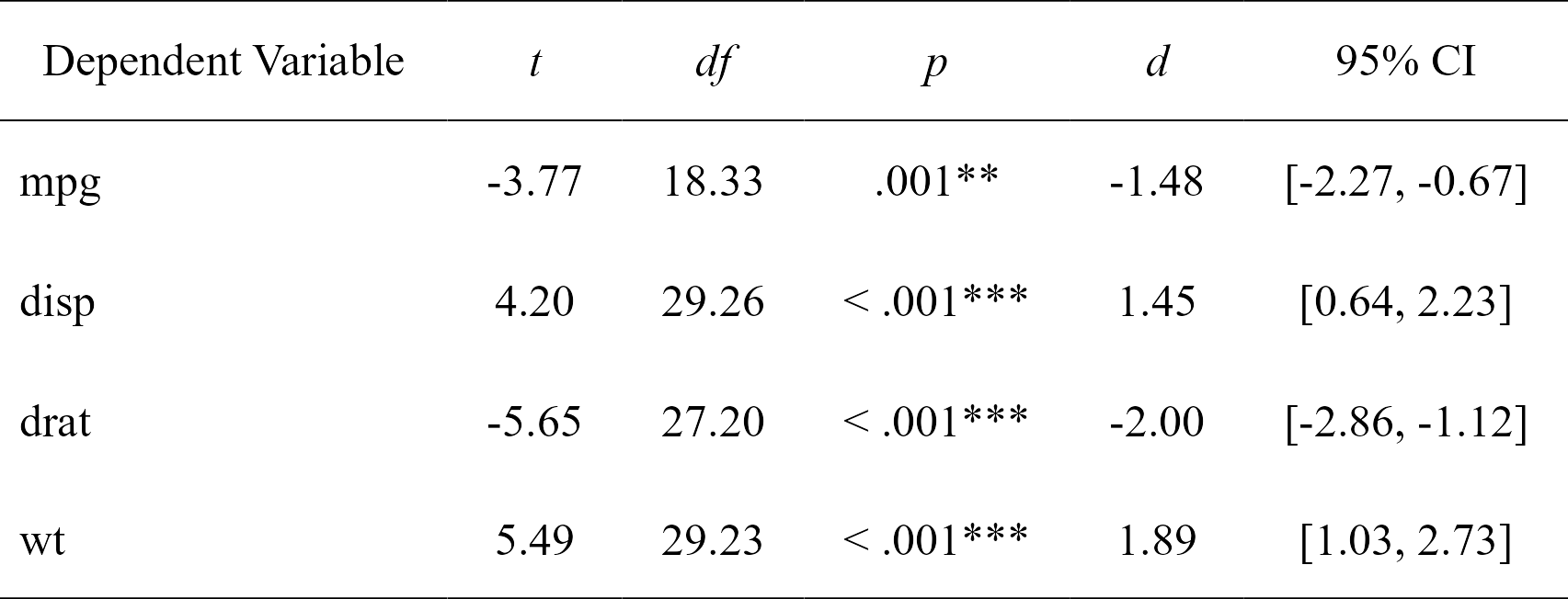
# Open in Word for quick copy-pasting
print(my_table, preview = "docx")

# Or save to Word
flextable::save_as_docx(t_table, path = "D:/R treasures/t_tests.docx")
Full tutorial: https://rempsyc.remi-theriault.com/articles/t-test
nice_contrastsEasily compute regression with planned contrast analyses (pairwise comparisons similar to t-tests but more powerful when more than 2 groups), and format in publication-ready format. Supports multiple dependent variables at once (but supports only three groups for the moment). In this particular case, the confidence intervals are bootstraped around the Cohen’s d.
contrasts <- nice_contrasts(
  data = mtcars,
  response = c("mpg", "disp"),
  group = "cyl",
  covariates = "hp"
)
contrasts
#>   Dependent Variable  Comparison df         t              p         d
#> 1                mpg cyl4 - cyl6 28  3.640418 0.001092088865  2.147244
#> 2                mpg cyl4 - cyl8 28  3.663188 0.001028617005  3.587739
#> 3                mpg cyl6 - cyl8 28  1.290359 0.207480642577  1.440495
#> 4               disp cyl4 - cyl6 28 -2.703423 0.011534398020 -1.514296
#> 5               disp cyl4 - cyl8 28 -6.040561 0.000001640986 -4.803022
#> 6               disp cyl6 - cyl8 28 -4.861413 0.000040511099 -3.288726
#>     CI_lower   CI_upper
#> 1  1.3531871  3.1223071
#> 2  2.7156109  4.4756393
#> 3  0.8435009  1.9939088
#> 4 -2.2636521 -0.8826532
#> 5 -5.8560355 -3.7464170
#> 6 -4.2833778 -2.2040887
# Format contrasts results
nice_table(contrasts, highlight = .001)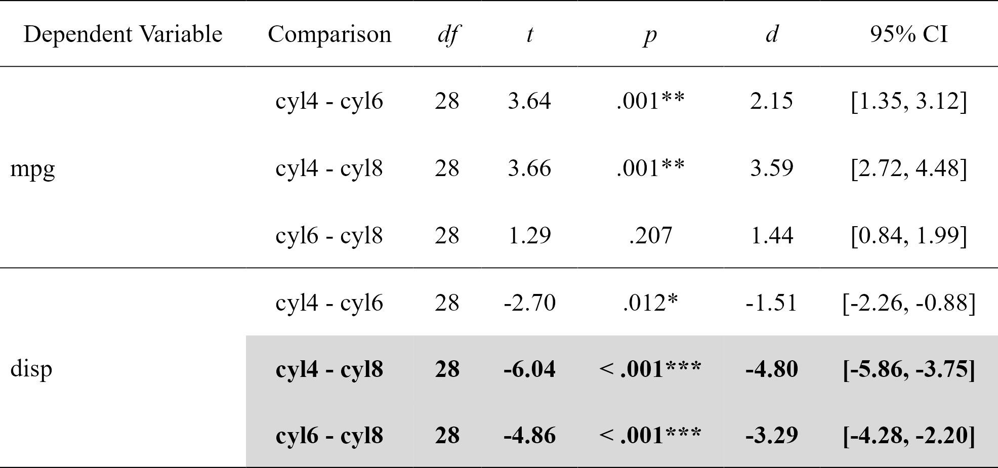
Full tutorial: https://rempsyc.remi-theriault.com/articles/contrasts
nice_modEasily compute moderation analyses, with effect sizes, and format in publication-ready format. Supports multiple dependent variables and covariates at once.
moderations <- nice_mod(
  data = mtcars,
  response = c("mpg", "disp"),
  predictor = "gear",
  moderator = "wt"
)
moderations
#>   Model Number Dependent Variable Predictor df           B          t
#> 1            1                mpg      gear 28 -0.08718042 -0.7982999
#> 2            1                mpg        wt 28 -0.94959988 -8.6037724
#> 3            1                mpg   gear:wt 28 -0.23559962 -2.1551077
#> 4            2               disp      gear 28 -0.07488985 -0.6967831
#> 5            2               disp        wt 28  0.83273987  7.6662883
#> 6            2               disp   gear:wt 28 -0.08758665 -0.8140664
#>                   p         sr2     CI_lower   CI_upper
#> 1 0.431415645312884 0.004805465 0.0000000000 0.02702141
#> 2 0.000000002383144 0.558188818 0.3142326391 0.80214500
#> 3 0.039899695159515 0.035022025 0.0003502202 0.09723370
#> 4 0.491683361920264 0.003546038 0.0000000000 0.02230154
#> 5 0.000000023731710 0.429258143 0.1916386492 0.66687764
#> 6 0.422476456495512 0.004840251 0.0000000000 0.02679265
# Format moderation results
nice_table(moderations, highlight = TRUE)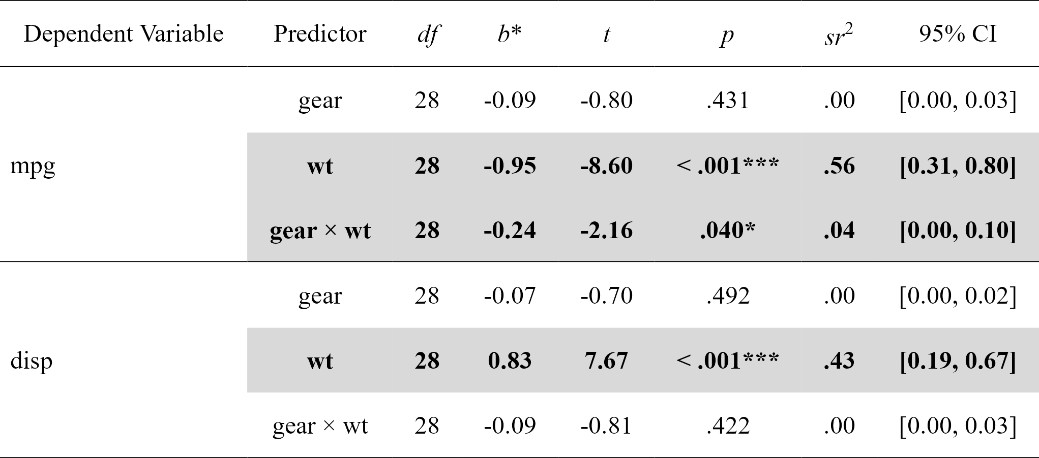
Full tutorial: https://rempsyc.remi-theriault.com/articles/moderation
nice_lmFor more complicated models not supported by nice_mod,
one can define the model in the traditional way and feed it to
nice_lm instead. Supports multiple lm models
as well.
model1 <- lm(mpg ~ cyl + wt * hp, mtcars)
model2 <- lm(qsec ~ disp + drat * carb, mtcars)
mods <- nice_lm(list(model1, model2), standardize = TRUE)
mods
#>   Model Number Dependent Variable Predictor df          B          t
#> 1            1                mpg       cyl 27 -0.1082286 -0.7180977
#> 2            1                mpg        wt 27 -0.6230206 -5.7013627
#> 3            1                mpg        hp 27 -0.2874898 -2.4045781
#> 4            1                mpg     wt:hp 27  0.2875867  3.2329593
#> 5            2               qsec      disp 27 -0.4315891 -1.9746464
#> 6            2               qsec      drat 27 -0.3337401 -1.5296603
#> 7            2               qsec      carb 27 -0.5092480 -3.3234897
#> 8            2               qsec drat:carb 27 -0.2307906 -1.0825727
#>                p         sr2     CI_lower   CI_upper
#> 1 0.478865160370 0.002159615 0.0000000000 0.01306786
#> 2 0.000004663587 0.136134000 0.0218243033 0.25044370
#> 3 0.023318649649 0.024215142 0.0002421514 0.06327779
#> 4 0.003221753406 0.043773344 0.0004377334 0.09898662
#> 5 0.058616844828 0.070256689 0.0000000000 0.19796621
#> 6 0.137733654712 0.042159840 0.0000000000 0.14133523
#> 7 0.002563609014 0.199020425 0.0019902043 0.40691582
#> 8 0.288572032972 0.021116556 0.0000000000 0.09136014
# Format moderation results
nice_table(mods, highlight = TRUE)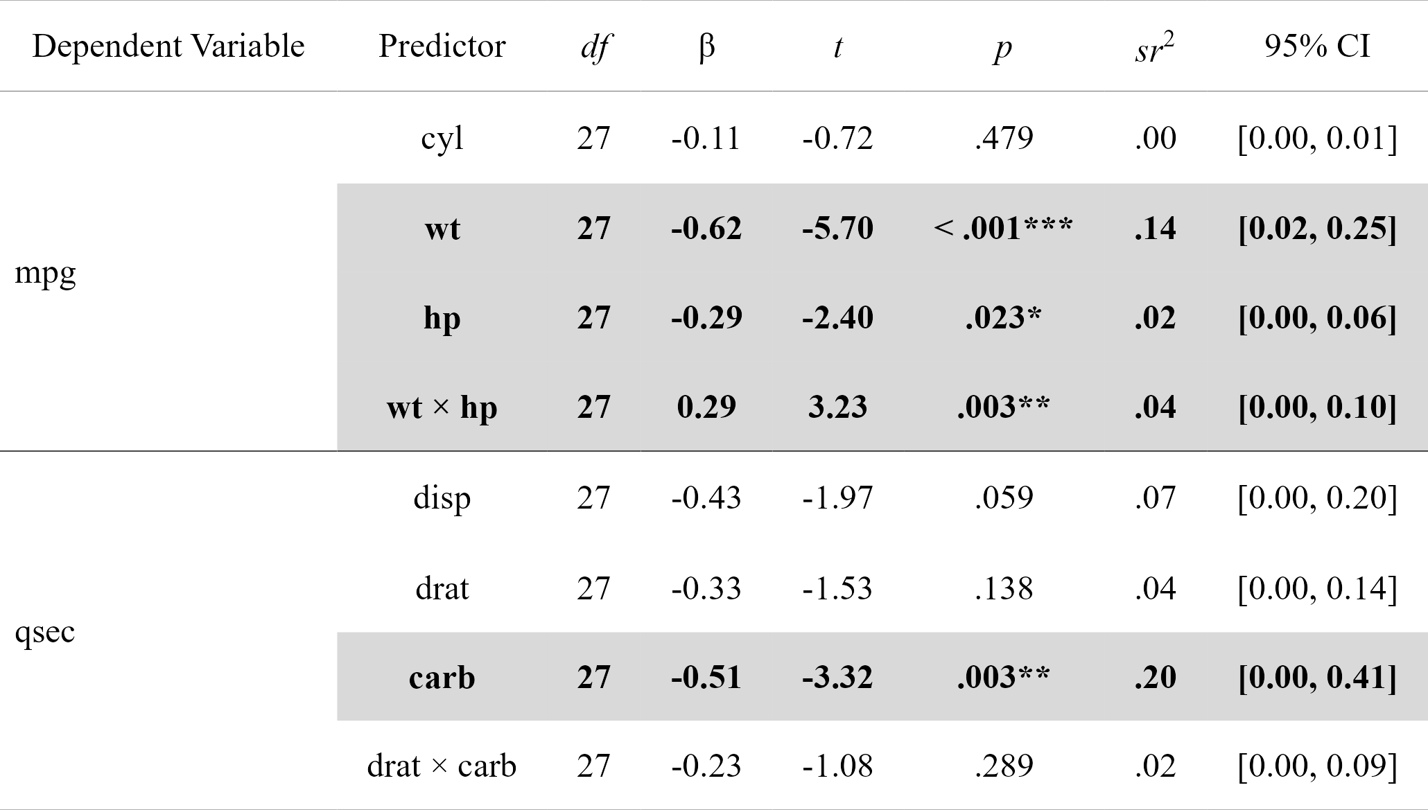
Full tutorial: https://rempsyc.remi-theriault.com/articles/moderation
nice_slopesEasily compute simple slopes in moderation analysis, with effect sizes, and format in publication-ready format. Supports multiple dependent variables and covariates at once.
simple.slopes <- nice_slopes(
  data = mtcars,
  response = c("mpg", "disp"),
  predictor = "gear",
  moderator = "wt"
)
simple.slopes
#>   Model Number Dependent Variable Predictor (+/-1 SD) df           B          t
#> 1            1                mpg       gear (LOW-wt) 28  0.14841920  1.0767040
#> 2            1                mpg      gear (MEAN-wt) 28 -0.08718042 -0.7982999
#> 3            1                mpg      gear (HIGH-wt) 28 -0.32278004 -1.9035367
#> 4            2               disp       gear (LOW-wt) 28  0.01269680  0.0935897
#> 5            2               disp      gear (MEAN-wt) 28 -0.07488985 -0.6967831
#> 6            2               disp      gear (HIGH-wt) 28 -0.16247650 -0.9735823
#>            p           sr2 CI_lower    CI_upper
#> 1 0.29080233 0.00874170174        0 0.038860523
#> 2 0.43141565 0.00480546484        0 0.027021406
#> 3 0.06729622 0.02732283901        0 0.081796622
#> 4 0.92610159 0.00006397412        0 0.002570652
#> 5 0.49168336 0.00354603816        0 0.022301536
#> 6 0.33860037 0.00692298820        0 0.033253212
# Format simple slopes results
nice_table(simple.slopes)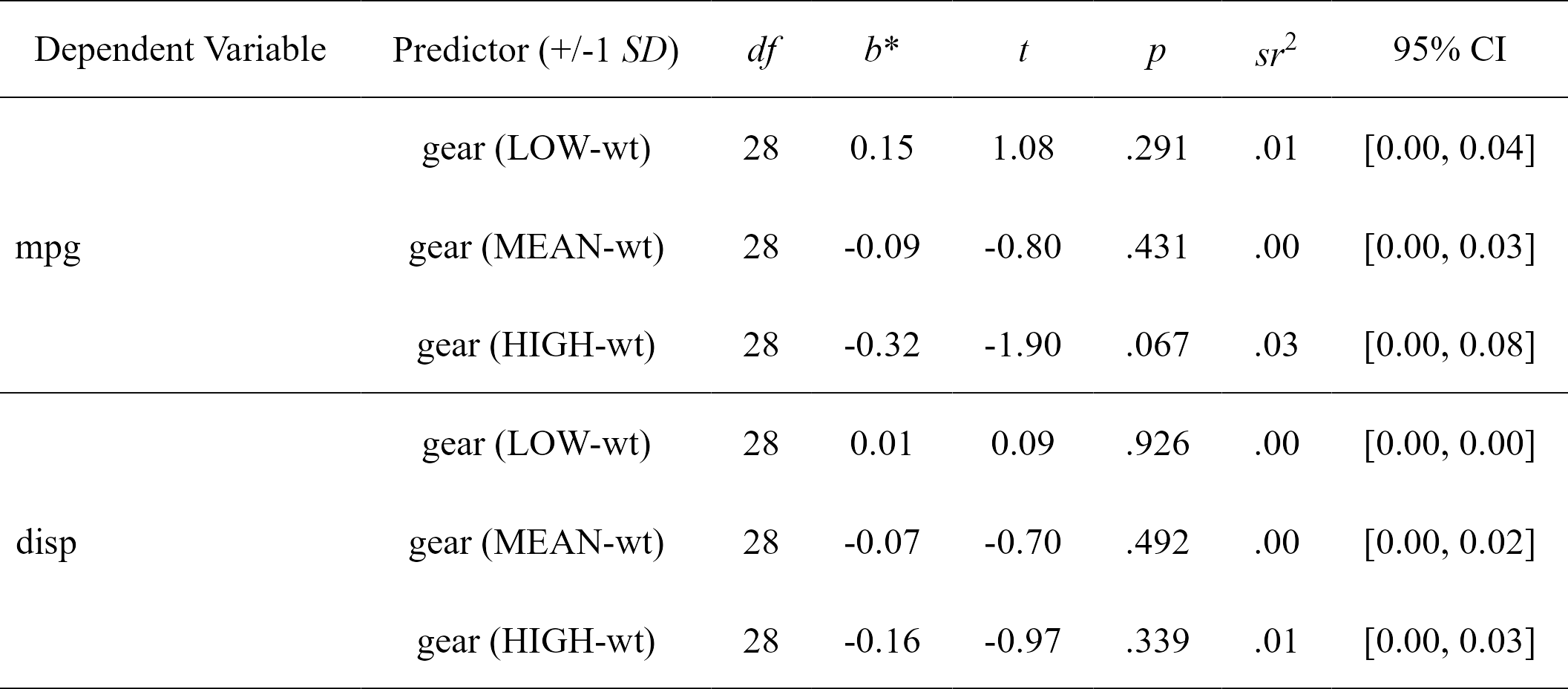
Full tutorial: https://rempsyc.remi-theriault.com/articles/moderation
nice_lm_slopesFor more complicated models not supported by
nice_slopes, one can define the model in the traditional
way and feed it to nice_lm_slopes instead. Supports
multiple lm models as well, but the predictor and moderator
need to be the same for these models (the dependent variable can
change).
model1 <- lm(mpg ~ gear * wt, mtcars)
model2 <- lm(disp ~ gear * wt, mtcars)
my.models <- list(model1, model2)
simple.slopes <- nice_lm_slopes(my.models, predictor = "gear", moderator = "wt", standardize = TRUE)
simple.slopes
#>   Model Number Dependent Variable Predictor (+/-1 SD) df           B          t
#> 1            1                mpg       gear (LOW-wt) 28  0.14841920  1.0767040
#> 2            1                mpg      gear (MEAN-wt) 28 -0.08718042 -0.7982999
#> 3            1                mpg      gear (HIGH-wt) 28 -0.32278004 -1.9035367
#> 4            2               disp       gear (LOW-wt) 28  0.01269680  0.0935897
#> 5            2               disp      gear (MEAN-wt) 28 -0.07488985 -0.6967831
#> 6            2               disp      gear (HIGH-wt) 28 -0.16247650 -0.9735823
#>            p           sr2 CI_lower    CI_upper
#> 1 0.29080233 0.00874170174        0 0.038860523
#> 2 0.43141565 0.00480546484        0 0.027021406
#> 3 0.06729622 0.02732283901        0 0.081796622
#> 4 0.92610159 0.00006397412        0 0.002570652
#> 5 0.49168336 0.00354603816        0 0.022301536
#> 6 0.33860037 0.00692298820        0 0.033253212
# Format simple slopes results
nice_table(simple.slopes)
Full tutorial: https://rempsyc.remi-theriault.com/articles/moderation
All plots can be saved with the ggplot2::ggsave()
function. They are ggplot2 objects so can be modified as
such.
nice_violinMake nice violin plots easily with 95% bootstrapped confidence intervals.
nice_violin(
  data = ToothGrowth,
  group = "dose",
  response = "len",
  xlabels = c("Low", "Medium", "High"),
  comp1 = 1,
  comp2 = 3,
  has.d = TRUE,
  d.y = 30
)
# Save plot
ggplot2::ggsave("niceplot.pdf",
  width = 7, height = 7, unit = "in",
  dpi = 300, path = "D:/R treasures/"
)
Full tutorial: https://rempsyc.remi-theriault.com/articles/violin
nice_scatterMake nice scatter plots easily.
nice_scatter(
  data = mtcars,
  predictor = "wt",
  response = "mpg",
  has.confband = TRUE,
  has.r = TRUE,
  has.p = TRUE
)
nice_scatter(
  data = mtcars,
  predictor = "wt",
  response = "mpg",
  group = "cyl",
  has.confband = TRUE
)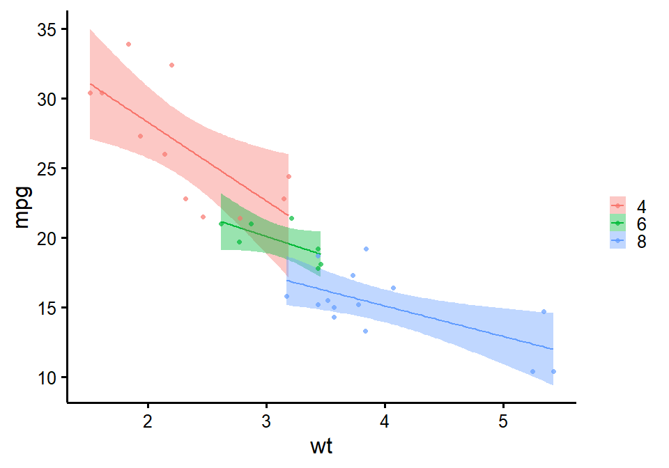
Full tutorial: https://rempsyc.remi-theriault.com/articles/scatter
plot_means_over_timeMake nice plots of means over time, usually for randomized controlled trials with several groups over several time measurements. Error bars represent 95% confidence intervals adjusted for within-subject variance as by the method of Morey (2008).
data <- mtcars
names(data)[6:3] <- paste0("T", 1:4, "_some-time-variable")

plot_means_over_time(
  data = data,
  response = names(data)[6:3],
  group = "cyl",
  groups.order = "decreasing",
  significance_bars_x = c(3.15, 4.15),
  significance_stars = c("*", "***"),
  significance_stars_x = c(3.25, 4.35),
  # significance_stars_y: List with structure: list(c("group1", "group2", time))
  significance_stars_y = list(c("4", "8", time = 3),
                              c("4", "8", time = 4)))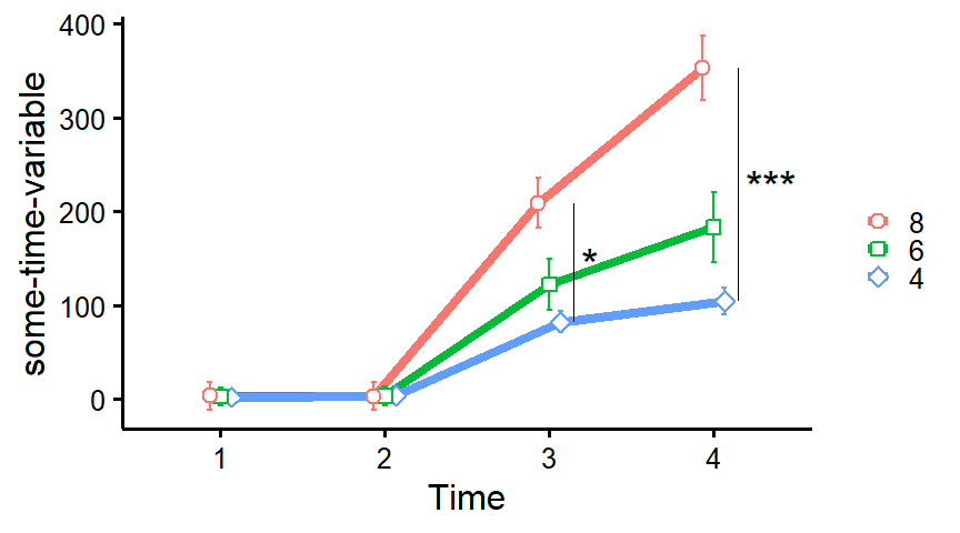
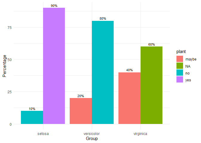
grouped_bar_chartMake nice plots of means over time, usually for randomized controlled trials with several groups over several time measurements. Error bars represent 95% confidence intervals adjusted for within-subject variance as by the method of Morey (2008).
iris2 <- iris
iris2$plant <- c(
  rep("yes", 45),
  rep("no", 45),
  rep("maybe", 30),
  rep("NA", 30)
)
grouped_bar_chart(
  data = iris2,
  response = "plant",
  group = "Species"
)
overlap_circleInterpolating the Inclusion of the Other in the Self Scale (self-other merging) easily.
# Score of 3.5 (25% overlap)
overlap_circle(3.5)
# Score of 6.84 (81.8% overlap)
overlap_circle(6.84)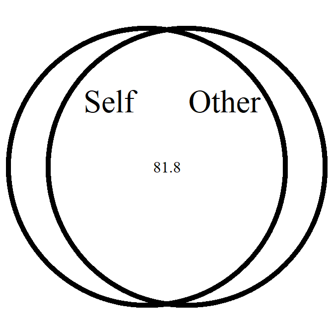
Full tutorial: https://rempsyc.remi-theriault.com/articles/circles
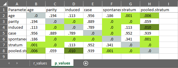
cormatrix_excelEasily output a correlation matrix and export it to Microsoft Excel, with the first row and column frozen, and correlation coefficients colour-coded based on their effect size (0.0-0.2: small (pink/light blue); 0.2-0.4: medium (orange/blue); 0.4-1.0: large (red/dark blue)).
cormatrix_excel(
  data = infert,
  filename = "cormatrix1",
  select = c(
    "age", "parity", "induced", "case", "spontaneous",
    "stratum", "pooled.stratum"
  )
)
#> # Correlation Matrix (pearson-method)
#>
#> Parameter      |      age |   parity |  induced |     case | spontaneous |  stratum | pooled.stratum
#> ----------------------------------------------------------------------------------------------------
#> age            |          |     0.08 |    -0.10 | 3.53e-03 |       -0.08 | -0.21*** |        -0.17**
#> parity         |     0.08 |          |  0.45*** | 8.91e-03 |     0.31*** | -0.31*** |           0.12
#> induced        |    -0.10 |  0.45*** |          |     0.02 |    -0.27*** |    -0.10 |          0.16*
#> case           | 3.53e-03 | 8.91e-03 |     0.02 |          |     0.36*** | 3.83e-03 |       4.86e-03
#> spontaneous    |    -0.08 |  0.31*** | -0.27*** |  0.36*** |             |     0.06 |        0.21***
#> stratum        | -0.21*** | -0.31*** |    -0.10 | 3.83e-03 |        0.06 |          |        0.75***
#> pooled.stratum |  -0.17** |     0.12 |    0.16* | 4.86e-03 |     0.21*** |  0.75*** |
#>
#> p-value adjustment method: none
#>
#>
#>  [Correlation matrix 'cormatrix1.xlsx' has been saved to working directory (or where specified).]
#> NULL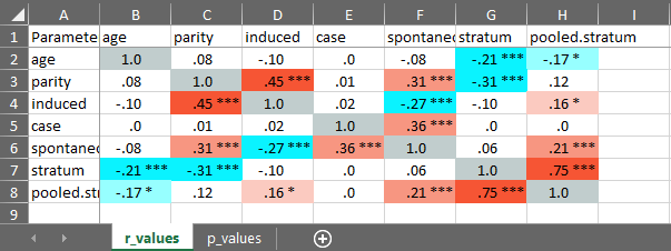
nice_naNicely reports NA values according to existing guidelines (i.e, reporting absolute or percentage of item-based missing values, plus each scale’s maximum amount of missing values for a given participant). Accordingly, allows specifying a list of columns representing questionnaire items to produce a questionnaire-based report of missing values.
# Create synthetic data frame for the demonstration
set.seed(50)
df <- data.frame(
  scale1_Q1 = c(sample(c(NA, 1:6), replace = TRUE), NA, NA),
  scale1_Q2 = c(sample(c(NA, 1:6), replace = TRUE), NA, NA),
  scale1_Q3 = c(sample(c(NA, 1:6), replace = TRUE), NA, NA),
  scale2_Q1 = c(sample(c(NA, 1:6), replace = TRUE), NA, NA),
  scale2_Q2 = c(sample(c(NA, 1:6), replace = TRUE), NA, NA),
  scale2_Q3 = c(sample(c(NA, 1:6), replace = TRUE), NA, NA),
  scale3_Q1 = c(sample(c(NA, 1:6), replace = TRUE), NA, NA),
  scale3_Q2 = c(sample(c(NA, 1:6), replace = TRUE), NA, NA),
  scale3_Q3 = c(sample(c(NA, 1:6), replace = TRUE), NA, NA)
)

# Then select your scales by name
nice_na(df, scales = c("scale1", "scale2", "scale3"))
#>                   var items na cells na_percent na_max na_max_percent all_na
#> 1 scale1_Q1:scale1_Q3     3  6    27      22.22      3            100      2
#> 2 scale2_Q1:scale2_Q3     3  9    27      33.33      3            100      2
#> 3 scale3_Q1:scale3_Q3     3  8    27      29.63      3            100      2
#> 4               Total     9 23    81      28.40      9            100      2

# Or whole dataframe
nice_na(df)
#>                   var items na cells na_percent na_max na_max_percent all_na
#> 1 scale1_Q1:scale3_Q3 9 23 81 28.4 9 100 2extract_duplicatesExtracts ALL duplicates (including the first one, contrary to
duplicated or dplyr::distinct) to a data frame
for visual inspection.
df1 <- data.frame(
  id = c(1, 2, 3, 1, 3),
  item1 = c(NA, 1, 1, 2, 3),
  item2 = c(NA, 1, 1, 2, 3),
  item3 = c(NA, 1, 1, 2, 3)
)
df1
#>   id item1 item2 item3
#> 1  1    NA    NA    NA
#> 2  2     1     1     1
#> 3  3     1     1     1
#> 4  1     2     2     2
#> 5  3     3     3     3

extract_duplicates(df1, id = "id")
#>   Row id item1 item2 item3 count_na
#> 1   1  1    NA    NA    NA        3
#> 2   4  1     2     2     2        0
#> 3   3  3     1     1     1        0
#> 4 5 3 3 3 3 0best_duplicateExtracts the “best” duplicate: the one with the fewer number of missing values (in case of ties, picks the first one).
best_duplicate(df1, id = "id")
#> (2 duplicates removed)
#>   id item1 item2 item3
#> 1  1     2     2     2
#> 2  2     1     1     1
#> 3 3 1 1 1scale_madScale and center (“standardize”) data based on the median and median absolute deviation (MAD).
scale_mad(mtcars$mpg)
#>  [1]  0.33262558  0.33262558  0.66525116  0.40654238 -0.09239599 -0.20327119
#>  [7] -0.90548075  0.96091834  0.66525116  0.00000000 -0.25870878 -0.51741757
#> [13] -0.35110478 -0.73916796 -1.62616950 -1.62616950 -0.83156395  2.43925425
#> [19]  2.06967028  2.71644224  0.42502157 -0.68373036 -0.73916796 -1.09027273
#> [25]  0.00000000  1.49681511  1.25658552  2.06967028 -0.62829276  0.09239599
#> [31] -0.77612635 0.40654238find_madIdentify outliers based on (e.g.,) 3 median absolute deviations (MAD) from the median.
find_mad(data = mtcars, col.list = names(mtcars)[c(1:7, 10:11)], criteria = 3)
#> 2 outlier(s) based on 3 median absolute deviations for variable(s):
#>  mpg, cyl, disp, hp, drat, wt, qsec, gear, carb
#>
#> Outliers per variable:
#>
#> $qsec
#>   Row qsec_mad
#> 1   9 3.665557
#>
#> $carb
#>   Row carb_mad
#> 1 31 4.046945winsorize_madWinsorize outliers based on (e.g.,) 3 median absolute deviations (MAD).
winsorize_mad(mtcars$qsec, criteria = 3)
#>  [1] 16.46000 17.02000 18.61000 19.44000 17.02000 20.22000 15.84000 20.00000
#>  [9] 21.95765 18.30000 18.90000 17.40000 17.60000 18.00000 17.98000 17.82000
#> [17] 17.42000 19.47000 18.52000 19.90000 20.01000 16.87000 17.30000 15.41000
#> [25] 17.05000 18.90000 16.70000 16.90000 14.50000 15.50000 14.60000 18.60000nice_reverseEasily recode scores (reverse-score), typically for questionnaire answers.
# Reverse score of 5 with a maximum score of 5
nice_reverse(5, 5)
#> [1] 1

# Reverse scores with maximum = 4 and minimum = 0
nice_reverse(1:4, 4, min = 0)
#> [1] 3 2 1 0

# Reverse scores with maximum = 3 and minimum = -3
nice_reverse(-3:3, 3, min = -3)
#> [1] 3 2 1 0 -1 -2 -3format_valueEasily format p or r values. Note: converts to
character class for use in figures or manuscripts to
accommodate e.g., “< .001”.
format_p(0.0041231)
#> [1] ".004"
format_p(t.tests$p)
#> [1] ".001"   "< .001" "< .001" "< .001"
format_r(moderations$sr2)
#> [1] ".00" ".56" ".04" ".00" ".43" ".00"
format_d(t.tests$d)
#> [1] "-1.48" "1.45" "-2.00" "1.89"nice_randomizeRandomize easily with different designs.
# Specify design, number of conditions, number of participants, and names of conditions:
nice_randomize(
  design = "between", Ncondition = 4, n = 8,
  condition.names = c("BP", "CX", "PZ", "ZL")
)
#>   id Condition
#> 1  1        ZL
#> 2  2        BP
#> 3  3        PZ
#> 4  4        CX
#> 5  5        CX
#> 6  6        PZ
#> 7  7        BP
#> 8  8        ZL

# Within-Group Design
nice_randomize(
  design = "within", Ncondition = 3, n = 3,
  condition.names = c("SV", "AV", "ST")
)
#>   id    Condition
#> 1  1 SV - AV - ST
#> 2  2 AV - ST - SV
#> 3  3 AV - SV - ST
Full tutorial: https://rempsyc.remi-theriault.com/articles/randomize
nice_assumptionsTest linear regression assumptions easily with a nice summary table.
# Create regression model
model <- lm(mpg ~ wt * cyl + gear, data = mtcars)
# View results
View(nice_assumptions(model))
Full tutorial: https://rempsyc.remi-theriault.com/articles/assumptions
nice_normalityEasily make nice density and QQ plots per-group.
nice_normality(
  data = iris,
  variable = "Sepal.Length",
  group = "Species",
  grid = FALSE,
  shapiro = TRUE,
  histogram = TRUE
)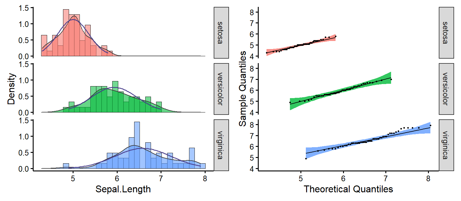
Full tutorial: https://rempsyc.remi-theriault.com/articles/assumptions
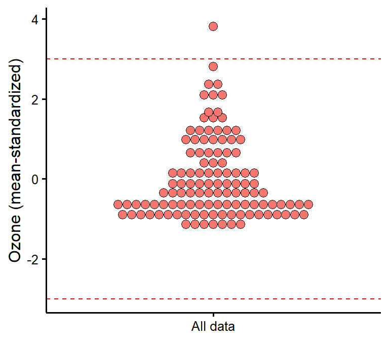
plot_outliersVisually check outliers based on (e.g.) +/- 3 MAD (median absolute deviations) or SD (standard deviations).
plot_outliers(airquality,
  group = "Month",
  response = "Ozone"
)
plot_outliers(airquality,
  response = "Ozone",
  method = "sd"
)
Full tutorial: https://rempsyc.remi-theriault.com/articles/assumptions
nice_varObtain variance per group as well as check for the rule of thumb of one group having variance four times bigger than any of the other groups.
nice_var(
  data = iris,
  variable = "Sepal.Length",
  group = "Species"
)
#>        Species Setosa Versicolor Virginica Variance.ratio Criteria
#> 1 Sepal.Length  0.124      0.266     0.404            3.3        4
#>   Heteroscedastic
#> 1           FALSE
Full tutorial: https://rempsyc.remi-theriault.com/articles/assumptions
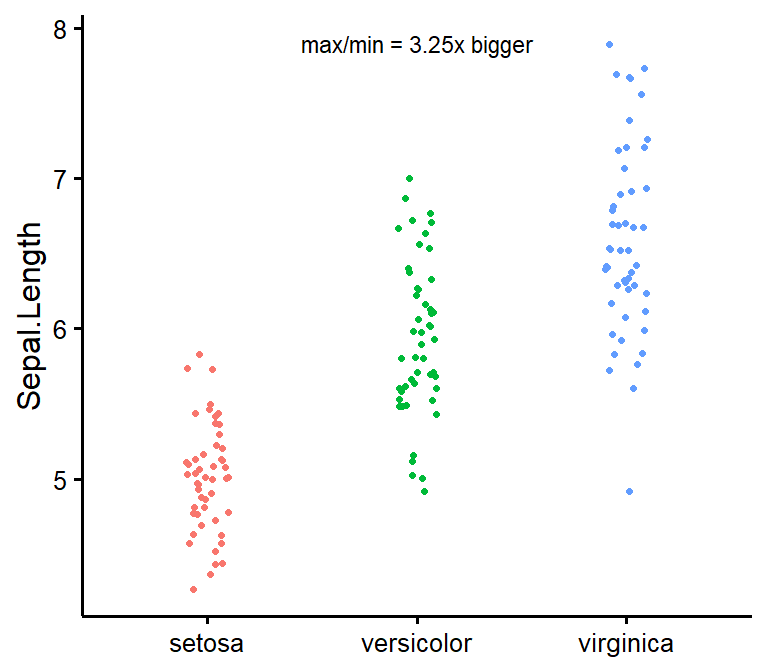
nice_varplotAttempt to visualize variance per group.
nice_varplot(
  data = iris,
  variable = "Sepal.Length",
  group = "Species"
)
Full tutorial: https://rempsyc.remi-theriault.com/articles/assumptions
lavaanExtraFor an alternative, vector-based syntax to lavaan (a
latent variable analysis/structural equation modeling package), as well
as other convenience functions such as naming paths and defining
indirect links automatically, see my other package,
lavaanExtra.
https://lavaanExtra.remi-theriault.com/
Thank you for your support. You can support me and this package here: https://github.com/sponsors/rempsyc