
![]()
![]()
Performs softmax regression for ordered outcomes under the Harville and Henery models.
– Steven E. Pav, shabbychef@gmail.com
This package can be installed from CRAN, via drat, or from github:
# via CRAN:
install.packages("ohenery")
# via drat:
if (require(drat)) {
    drat:::add("shabbychef")
    install.packages("ohenery")
}
# get snapshot from github (may be buggy)
if (require(devtools)) {
  install_github('shabbychef/ohenery')
}
The softmax regression generalizes logistic regression, wherein only one of two possible outcomes is observed, to the case where one of many possible outcomes is observed. As in logistic regression, one models the log odds of each outcome as a linear function of some independent variables. Moreover, a softmax regression allows one to model data from events where the number of possible outcomes differs.
Some examples where one might apply a softmax regression:
Note that in the examples illustrated above, one might be better served by modeling some continuous outcome, instead of modeling the winner. For example, one might model the speed of each racer, or the number of votes each film garnered, or the total amount of rain each city experienced. Discarding this information in favor of modeling the binary outcome is likely to cause a loss of statistical power, and is generally discouraged. However, in some cases the continuous outcome is not observed, as in the case of the Best Picture awards, or in horse racing where finishing times are often not available. Softmax regression can be used in these cases.
The softmax regression can be further generalized to model the case
where one observes place information about participants. For example,
one might observe which of first through fifth place each sprinter
claims in each race.
Or one might only observe some limited information, like the Gold,
Silver and Bronze medal winners in an Olympic event.
There is more than one way to generalize the softmax to deal with ranked outcomes like these:
This package supports fitting softmax regressions under both models.
Here we use softmax regression to model the Best Picture winner odds as linear in some features: whether the film also was nominated for Best Director, Best Actor or Actress, or Best Film Editing, as well as genre designations for Drama, Romance and Comedy. We only observe the winner of the Best Picture award, and not runners-up, so we weight the first place finisher with a one, and all others with a zero. This seems odd, but it ensures that the regression does not try to compare model differences between the runners-up. We find the strongest absolute effect on odds from the Best Director and Film Editing co-nomination variables.
library(ohenery)
library(dplyr)
library(magrittr)
data(best_picture)
best_picture %<>%
  mutate(place=ifelse(winner,1,2)) %>%
  mutate(weight=ifelse(winner,1,0))

fmla <- place ~ nominated_for_BestDirector + nominated_for_BestActor + nominated_for_BestActress + nominated_for_BestFilmEditing + Drama + Romance + Comedy

osmod <- harsm(fmla,data=best_picture,group=year,weights=weight)
print(osmod)
## --------------------------------------------
## Maximum Likelihood estimation
## BFGS maximization, 59 iterations
## Return code 0: successful convergence
## Log-Likelihood: -92
## 7 free parameters
## Estimates:
## Estimate Std. error t value Pr(> t)
## nominated_for_BestDirectorTRUE 3.294 0.850 3.88 0.00011 ***
## nominated_for_BestActorTRUE 1.003 0.316 3.18 0.00149 **
## nominated_for_BestActressTRUE 0.048 0.348 0.14 0.89048
## nominated_for_BestFilmEditingTRUE 1.949 0.399 4.88 1e-06 ***
## Drama -0.659 0.605 -1.09 0.27580
## Romance 0.521 0.974 0.53 0.59291
## Comedy 1.317 1.013 1.30 0.19333
## ---
## Signif. codes: 0 '***' 0.001 '**' 0.01 '*' 0.05 '.' 0.1 ' ' 1
## --------------------------------------------
## R2: 0.77
## --------------------------------------------Here we use the predict method to get back predictions
under the Harville model produced above. Three different types of
prediction are supported:
We do not currently have the ability to compute the expected rank under the Henery model, as it is too computationally intensive. (File an issue if this is important.)
prd <- best_picture %>%
  mutate(prd_erank=as.numeric(predict(osmod,newdata=.,group=year,type='erank',na.action=na.pass))) %>%
  mutate(prd_eta=as.numeric(predict(osmod,newdata=.,group=year,type='eta'))) %>%
mutate(prd_mu=as.numeric(predict(osmod,newdata=.,group=year,type='mu'))) The package is bundled with a dataset of three weeks of thoroughbred and harness race results from tracks around the world. First, let us compare the ‘consensus odds’, as computed from the win pool size, with the probability of winning a race. This is usually plotted as the empirical win probability over horses grouped by their consensus win probability.
We present this plot below. Clearly visible are the ‘longshot bias’ and ‘sureshot bias’ (or favorite bias). The longshot bias is the effect where longshots are overbet, resulting in elevated consensus odds. This appears as the point off the line in the lower left. One can think of these as points which were moved to the right of the plot from a point on the diagonal by overbetting. The sureshot bias is the complementary effect where favorites to win are underbet, effectively shifting the points to the left.
library(ohenery)
library(dplyr)
library(magrittr)
library(ggplot2)

data(race_data)

ph <- race_data %>%
  group_by(EventId) %>%
    mutate(mu0=WN_pool / sum(WN_pool)) %>%
  ungroup() %>%
  mutate(mubkt=cut(mu0,c(0,10^seq(-2,0,length.out=14)),include.lowest=TRUE)) %>%
  mutate(tookfirst=as.numeric(coalesce(Finish==1,FALSE))) %>%
  group_by(mubkt) %>%
    summarize(winprop=mean(tookfirst),
              medmu=median(mu0),
              nrace=length(unique(EventId)),
              nhorse=n()) %>%
  ungroup() %>%
  ggplot(aes(medmu,winprop)) +
  geom_point(aes(size=nhorse)) +
  geom_abline(intercept=0,slope=1) +
  scale_x_log10(labels=scales::percent) +
  scale_y_log10(labels=scales::percent) +
  labs(x='consensus odds (from win pool)',
       y='empirical win probability',
       title='efficiency of the win pool')
print(ph)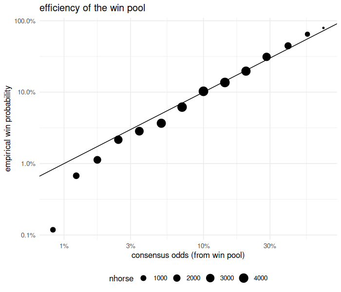
plot of chunk race_data_efficiency
Here we use softmax regression under the Harville model to capture the longshot and sureshot biases. Our model computes consensus odds as the inverse softmax function of the consensus probabilities, which are constructed from the win pool. We define a factor variable that captures longshot, sureshot, and ‘vanilla’ bets based on the win pool-implied probabilities. Here we are only concerned with the win probabilities, so we adapt a Harville model and weight only the winning finishers.
# because of na.action, make ties for fourth
df <- race_data %>%
  mutate(Outcome=coalesce(Finish,4L))

# create consensus odds eta0
df %<>%
  mutate(weights=coalesce(as.numeric(Finish==1),0) ) %>%
  group_by(EventId) %>%
    mutate(big_field=(n() >= 6)) %>%
    mutate(mu0=WN_pool / sum(WN_pool)) %>%
    mutate(eta0=inv_smax(mu0)) %>%
  ungroup() %>%
  dplyr::filter(big_field) %>%
  dplyr::filter(!is.na(eta0)) %>%
  mutate(bettype=factor(case_when(mu0 < 0.025 ~ 'LONGSHOT',
                                  mu0 > 0.50  ~ 'SURESHOT',
                                  TRUE        ~ 'VANILLA')))

# Harville Model with market efficiency
effmod <- harsm(Outcome ~ eta0:bettype,data=df,group=EventId,weights=weights)
print(effmod)
## --------------------------------------------
## Maximum Likelihood estimation
## BFGS maximization, 44 iterations
## Return code 0: successful convergence
## Log-Likelihood: -6862
## 3 free parameters
## Estimates:
## Estimate Std. error t value Pr(> t)
## eta0:bettypeLONGSHOT 1.2602 0.0977 12.9 <2e-16 ***
## eta0:bettypeSURESHOT 1.1896 0.0417 28.5 <2e-16 ***
## eta0:bettypeVANILLA 1.1158 0.0257 43.4 <2e-16 ***
## ---
## Signif. codes: 0 '***' 0.001 '**' 0.01 '*' 0.05 '.' 0.1 ' ' 1
## --------------------------------------------
## R2: 0.53
## --------------------------------------------We see that in this model the beta coefficient for consensus odds is around 1.12 for ‘vanilla’ bets, slightly higher for sure bets, and much higher for longshots. The interpretation is that long shots are relatively overbet, but that otherwise bets are nearly efficient.
One would like to make a correction to inefficiencies in the win pool by generalizing this idea to multiple cut points along the consensus probabilities. However, the softmax model works by tweaking the consensus odds; the odds translate into win probabilities in a way that depends on the other participants, and so there is no one curve.
The print display of the Harville softmax regression includes an ‘R-squared’ and sometimes a ‘delta R-squared’. The latter is only reported when an offset is used in the model. The R-squared is the improvement in spread in the predicted ranks from the model compared to the null model which assumes all log odds are equal. When an offset is given, the R-squared includes the offset, but a ‘delta’ R-squared is reported which gives the improvement in spread of predicted ranks over the model based on the offset:
# Harville Model with offset
offmod <- harsm(Outcome ~ offset(eta0) + bettype,data=df,group=EventId,weights=weights)
print(offmod)
## --------------------------------------------
## Maximum Likelihood estimation
## BFGS maximization, 25 iterations
## Return code 0: successful convergence
## Log-Likelihood: -6872
## 2 free parameters
## Estimates:
## Estimate Std. error t value Pr(> t)
## bettypeSURESHOT 0.816 0.150 5.43 5.5e-08 ***
## bettypeVANILLA 0.437 0.126 3.46 0.00054 ***
## ---
## Signif. codes: 0 '***' 0.001 '**' 0.01 '*' 0.05 '.' 0.1 ' ' 1
## --------------------------------------------
## R2: 0.1
## delR2: -0.86
## --------------------------------------------Unfortunately, the R-squareds are hard to interpret, and can sometimes give negative values. The softmax regression is not guaranteed to improve the residual sum of squared errors in the rank.
Here we fit a Henery model to the horse race data. Note that in the
data we only observe win, place, and show finishes, so we assign zero
weight to all other finishers.
Again this is so the regression does not attempt to model distinctions
between runners-up. Moreover, because of how na.action
works on the input data, the response variable has to be coalesced with
tie-breakers.
# because of na.action, make ties for fourth
df <- race_data %>%
  mutate(Outcome=coalesce(Finish,4L)) %>%
  mutate(weights=coalesce(as.numeric(Finish<=3),0) ) %>%  # w/p/s
  group_by(EventId) %>%
    mutate(big_field=(n() >= 5)) %>%
    mutate(mu0=WN_pool / sum(WN_pool)) %>%
    mutate(eta0=inv_smax(mu0)) %>%
  ungroup() %>%
  dplyr::filter(big_field) %>%
  dplyr::filter(!is.na(eta0)) %>%
  mutate(fac_age=cut(Age,c(0,3,5,7,Inf),include.lowest=TRUE)) %>%
  mutate(bettype=factor(case_when(mu0 < 0.025 ~ 'LONGSHOT',
                                  mu0 > 0.50  ~ 'SURESHOT',
                                  TRUE        ~ 'VANILLA')))

# Henery Model with ...
bigmod <- hensm(Outcome ~ eta0:bettype + fac_age,data=df,group=EventId,weights=weights,ngamma=3)
print(bigmod)
## --------------------------------------------
## Maximum Likelihood estimation
## BFGS maximization, 57 iterations
## Return code 0: successful convergence
## Log-Likelihood: -21720
## 8 free parameters
## Estimates:
## Estimate Std. error t value Pr(> t)
## fac_age(3,5] 0.2024 0.0697 2.90 0.0037 **
## fac_age(5,7] 0.1704 0.0794 2.14 0.0320 *
## fac_age(7,Inf] 0.1531 0.0848 1.80 0.0711 .
## eta0:bettypeLONGSHOT 1.5191 0.0641 23.70 <2e-16 ***
## eta0:bettypeSURESHOT 1.1096 0.0367 30.19 <2e-16 ***
## eta0:bettypeVANILLA 1.1107 0.0231 48.06 <2e-16 ***
## gamma2 0.7053 0.0215 32.84 <2e-16 ***
## gamma3 0.5274 0.0191 27.63 <2e-16 ***
## ---
## Signif. codes: 0 '***' 0.001 '**' 0.01 '*' 0.05 '.' 0.1 ' ' 1
## --------------------------------------------Note that the gamma coefficients are fit here as 0.71, 0.53. Values around 0.8 or smaller are typical. (In a future release it would probably make sense to make the gammas relative to the value 1, which would make it easier to reject the Harville model from the print summary.)
The package is bundled with a dataset of 100 years of Olympic Men’s Platform Diving Records, originally sourced by Randi Griffin and delivered on kaggle.
Here we convert the medal records into finishing places of 1, 2, 3 and 4 (no medal), add weights for the fitting, make a factor variable for age, factor the NOC (country) of the athlete. Because Platform Diving is a subjective competition, based on scores from judges, we investigate whether there is a ‘home field advantage’ by creating a Boolean variable indicating whether the athlete is representing the host nation.
We then fit a Henery model to the data. Note that the gamma terms come out very close to one, indicating the Harville model would be sufficient. The home field advantage does not appear significant in this analysis.
library(forcats)
data(diving)
fitdat <- diving %>%
  mutate(Finish=case_when(grepl('Gold',Medal)   ~ 1,
                          grepl('Silver',Medal) ~ 2,
                          grepl('Bronze',Medal) ~ 3,
                          TRUE ~ 4)) %>%
  mutate(weight=ifelse(Finish <= 3,1,0)) %>%
  mutate(cut_age=cut(coalesce(Age,22.0),c(12,19.5,21.5,22.5,25.5,99),include.lowest=TRUE)) %>%
  mutate(country=forcats::fct_relevel(forcats::fct_lump(factor(NOC),n=5),'Other')) %>%
  mutate(home_advantage=NOC==HOST_NOC)

hensm(Finish ~ cut_age + country + home_advantage,data=fitdat,weights=weight,group=EventId,ngamma=3)
## --------------------------------------------
## Maximum Likelihood estimation
## BFGS maximization, 43 iterations
## Return code 0: successful convergence
## Log-Likelihood: -214
## 12 free parameters
## Estimates:
## Estimate Std. error t value Pr(> t)
## cut_age(19.5,21.5] 0.0303 0.4185 0.07 0.94227
## cut_age(21.5,22.5] -0.7276 0.5249 -1.39 0.16565
## cut_age(22.5,25.5] 0.0950 0.3790 0.25 0.80199
## cut_age(25.5,99] -0.1838 0.4111 -0.45 0.65474
## countryGBR -0.6729 0.8039 -0.84 0.40258
## countryGER 1.0776 0.4960 2.17 0.02981 *
## countryMEX 0.7159 0.4744 1.51 0.13126
## countrySWE 0.6207 0.5530 1.12 0.26172
## countryUSA 2.3201 0.4579 5.07 4.1e-07 ***
## home_advantageTRUE 0.5791 0.4112 1.41 0.15904
## gamma2 1.0054 0.2853 3.52 0.00042 ***
## gamma3 0.9674 0.2963 3.26 0.00109 **
## ---
## Signif. codes: 0 '***' 0.001 '**' 0.01 '*' 0.05 '.' 0.1 ' ' 1
## --------------------------------------------The regression coefficients are fit by Maximum Likelihood Estimation,
and the maxLik package does the ‘heavy lifting’ of
estimating the variance-covariance of the coefficients. However, it is
not clear a priori that these error estimates are accurate,
since the individual outcomes in a given event are not independent: it
could be that the machinery for computing the Fisher Information matrix
is inaccurate. In fact, the help from maxLik warns that
this is on the user. This is especially concerning when the logistic
fits are used in situations where not all finishes are observed, and one
uses zero weights to avoid affecting the fits.
Here we will try to establish empirically that the inference is actually correct.
As the Harville model generalizes logistic regression, we should be
able to run a logistic regression problem through the harsm
function. Here we do that, testing data with exactly two participants
per event. The key observation is that the usual logistic regression
should be equivalent to the Harville form, but with independent
variables equal to the difference in independent variables for
the two participants. We find that the coefficients and
variance-covariance matrix are nearly identical. We believe the
differences are due to convergence criteria in the MLE fit.
library(dplyr)
nevent <- 10000
set.seed(1234)
adf <- data_frame(eventnum=floor(seq(1,nevent + 0.7,by=0.5))) %>%
  mutate(x=rnorm(n()),
         program_num=rep(c(1,2),nevent),
         intercept=as.numeric(program_num==1),
         eta=1.5 * x + 0.3 * intercept,
         place=ohenery::rsm(eta,g=eventnum))

# Harville model
modh <- harsm(place ~ intercept + x,data=adf,group=eventnum)

# the collapsed data.frame for glm
ddf <- adf %>%
  arrange(eventnum,program_num) %>%
  group_by(eventnum) %>%
    summarize(resu=as.numeric(first(place)==1),
              delx=first(x) - last(x),
              deli=first(intercept) - last(intercept)) %>%
  ungroup()

# glm logistic fit
modg <- glm(resu ~ delx + 1,data=ddf,family=binomial(link='logit'))

all.equal(as.numeric(coef(modh)),as.numeric(coef(modg)),tolerance=1e-4)
## [1] TRUEall.equal(as.numeric(vcov(modh)),as.numeric(vcov(modg)),tolerance=1e-4)## [1] TRUEprint(coef(modh))## intercept x
## 0.34 1.49print(coef(modg))## (Intercept) delx
## 0.34 1.49print(vcov(modh))## intercept x
## intercept 0.00071 0.00012
## x 0.00012 0.00091print(vcov(modg))## (Intercept) delx
## (Intercept) 0.00071 0.00012
## delx 0.00012 0.00091We now examine whether inference is correct in the case when weights are used to denote that some finishes are not observed. The first release of this package defaulted to using ‘normalized weights’ in the Harville and Henery fits. I believe this leads to an inflated Fisher Information that then causes the estimated variance-covariance matrix to be too small. I am changing the default in version 0.2.0 to fix this issue.
Here I generate some data, and fit to the Harville model, using weights to signify that we have only observed three of the 8 finishing places in each event. I compute the the estimate minus the true value, divided by the estimated standard error. I repeat this process many times. Asymptotically in sample size, this computed value should be a standard normal. I check by taking the standard deviation, and Q-Q plotting against standard normal. The results are consistent with correct inference.
library(dplyr)
nevent <- 5000
# 3 of 8 observed values.
wlim <- 3
nfield <- 8
beta <- 2
library(future.apply)
plan(multicore,workers=7)
set.seed(1234)
zvals <- future_replicate(500,{
  adf <- data_frame(eventnum=sort(rep(seq_len(nevent),nfield))) %>%
        mutate(x=rnorm(n()),
                     program_num=rep(seq_len(nfield),nevent),
                     eta=beta * x,
                     place=ohenery::rsm(eta,g=eventnum),
                     wts=as.numeric(place <= wlim))

    modo <- ohenery::harsm(place ~ x,data=adf,group=eventnum,weights=wts)
    as.numeric(coef(modo) - beta) / as.numeric(sqrt(vcov(modo)))
})
plan(sequential)

# this should be near 1
sd(zvals)
## [1] 0.98# QQ plot it
library(ggplot2)
ph <- data_frame(zvals=zvals) %>%
ggplot(aes(sample=zvals)) +
stat_qq(alpha=0.4) +
geom_abline(linetype=2,color='red') +
labs(title='putative z-values from Harville fits')
print(ph)
plot of chunk wted_zsims
The package supports regularization of coefficients in the estimation of the Harville and Henery models. When regularization is used, the objective that is maximized is \[ \log{L} - \sum_i w_i | \nu_{c_i} - z_i |^{p_i}, \] where \(\log{L}\) is the log likelihood, the \(w_i\) are regularization weights, \(z_i\) are the regularization “zeroes” (where the coefficients are shrunk to), \(p_i\) are the regularization powers, and \(c_i\) are the regularization indices. By use of these indices the regularization term can penalize the same coefficient with multiple powers, as in elasticnet. The \(\nu\) here are the coefficients \(\beta\) which are estimated in the Harville model or the \(\beta\) and the \(\gamma_2, \gamma_3, \ldots\) estimated in the Henery model, in that order.
An optional flag to “standardize” the regularization adjusts the \(w_i\) to be sensitive to the corresponding independent variable’s standard deviation. This allows the same regularization to be applied under a rescaling of units, and also makes it easier to penalize different coefficients at approximately the same scale. Note that it is not clear that the observed standard deviation is the right measure here, since what is important in the softmax fits is the diversity of a variable within a given match. That is, if there is a lot of variation across matches of some variable, but only a small amount within each match, the variable may have little apparent effect. Thus the standardization is not a perfect fix.
Here we illustrate regulariztion using the Diving data as above.
library(broom)
library(tidyr)
library(knitr)
# no regularization
mod0 <- hensm(Finish ~ cut_age + country + home_advantage,data=fitdat,weights=weight,group=EventId,ngamma=3)
# l2 regularization
mod0_l2 <- hensm(Finish ~ cut_age + country + home_advantage,data=fitdat,weights=weight,group=EventId,ngamma=3,
                            reg_wt=1,reg_power=2,reg_coef_idx=1:10,reg_zero=0)
# l1 regularization
mod0_l1 <- hensm(Finish ~ cut_age + country + home_advantage,data=fitdat,weights=weight,group=EventId,ngamma=3,
                            reg_wt=1,reg_power=1,reg_coef_idx=1:10,reg_zero=0)
# l1 & l2 regularization
mod0_l1l2 <- hensm(Finish ~ cut_age + country + home_advantage,data=fitdat,weights=weight,group=EventId,ngamma=3,
                                 reg_wt=1,reg_power=rep(c(1,2),each=10),reg_coef_idx=rep(1:10,2),reg_zero=0)

lapply(list(base=mod0,l1=mod0_l1,l2=mod0_l2,l1l2=mod0_l1l2),broom::tidy) %>%
    bind_rows(.id='model') %>%
    select(model,term,estimate) %>%
    tidyr::spread(key=model,value=estimate) %>%
knitr::kable(caption='Henery model fits with shrinkage on the betas.')| term | base | l1 | l1l2 | l2 |
|---|---|---|---|---|
| countryGBR | -0.67 | -0.26 | -0.17 | -0.31 |
| countryGER | 1.08 | 0.72 | 0.46 | 0.60 |
| countryMEX | 0.72 | 0.44 | 0.29 | 0.39 |
| countrySWE | 0.62 | 0.28 | 0.17 | 0.28 |
| countryUSA | 2.32 | 1.86 | 1.13 | 1.45 |
| cut_age(19.5,21.5] | 0.03 | 0.00 | 0.00 | -0.01 |
| cut_age(21.5,22.5] | -0.73 | -0.47 | -0.27 | -0.40 |
| cut_age(22.5,25.5] | 0.10 | 0.08 | 0.07 | 0.09 |
| cut_age(25.5,99] | -0.18 | -0.10 | -0.11 | -0.16 |
| gamma2 | 1.01 | 1.24 | 2.05 | 1.60 |
| gamma3 | 0.97 | 1.22 | 2.03 | 1.59 |
| home_advantageTRUE | 0.58 | 0.37 | 0.26 | 0.37 |
We now illustrate shrinkage of the \(\gamma\) as well; these are typically shrunk towards 1.
# no regularization
mod0 <- hensm(Finish ~ cut_age + country + home_advantage,data=fitdat,weights=weight,group=EventId,ngamma=3)
# l1 regularization
mod0_l1 <- hensm(Finish ~ cut_age + country + home_advantage,data=fitdat,weights=weight,group=EventId,ngamma=3,
                            reg_wt=1,reg_power=1,reg_coef_idx=11:12,reg_zero=1)

lapply(list(base=mod0,l1=mod0_l1),broom::tidy) %>%
    bind_rows(.id='model') %>%
    select(model,term,estimate) %>%
    tidyr::spread(key=model,value=estimate) %>%
    arrange(grepl('gamma',term),term) %>%
knitr::kable(caption='Henery model fits with shrinkage on the gammas only.')| term | base | l1 |
|---|---|---|
| countryGBR | -0.67 | -0.64 |
| countryGER | 1.08 | 1.07 |
| countryMEX | 0.72 | 0.71 |
| countrySWE | 0.62 | 0.62 |
| countryUSA | 2.32 | 2.30 |
| cut_age(19.5,21.5] | 0.03 | 0.02 |
| cut_age(21.5,22.5] | -0.73 | -0.74 |
| cut_age(22.5,25.5] | 0.10 | 0.09 |
| cut_age(25.5,99] | -0.18 | -0.19 |
| home_advantageTRUE | 0.58 | 0.58 |
| gamma2 | 1.01 | 1.00 |
| gamma3 | 0.97 | 1.00 |