![]()
![]()
A package designed to handle multiplexed imaging data in R, implementing normalization methods and quality metrics detailed in our paper here. Further information about the package, usage, the vignettes, and more can be found on CRAN.
To install from CRAN, use:
install.packages("mxnorm")You can install the development version from GitHub with:
# install.packages("devtools")
devtools::install_github("ColemanRHarris/mxnorm")This package imports lme4 (and its dependency
nloptr) which use CMake to build the packages.
To install CMake, please see here or select from the
following:
- yum install cmake          (Fedora/CentOS; inside a terminal)
- apt install cmake          (Debian/Ubuntu; inside a terminal).
- pacman -S cmake            (Arch Linux; inside a terminal).
- brew install cmake         (MacOS; inside a terminal with Homebrew)
- port install cmake         (MacOS; inside a terminal with MacPorts)
This package also uses the reticulate package to
interface with the scikit-learn Python package. Depending
on the user’s environment, sometimes
Python/conda/Miniconda is not detected,
producing an option like the following:
No non-system installation of Python could be found.
Would you like to download and install Miniconda?
Miniconda is an open source environment management system for Python.
See https://docs.conda.io/en/latest/miniconda.html for more details.

Would you like to install Miniconda? [Y/n]:
In this case, installing Miniconda within the R environment will
ensure that both Python and the scikit-image package are
properly installed. However, if you want to use a separate Python
installation, please respond N to this prompt and use
reticulate::py_config() to setup your Python environment.
Please also ensure that scikit-image is installed in your
desired Python environment via
pip install scikit-image.
Please report any issues, bugs, or problems with the software here: https://github.com/ColemanRHarris/mxnorm/issues. For any contributions, feel free to fork the package repository on GitHub or submit pull requests. Any other contribution questions and requests for support can be directed to the package maintainer Coleman Harris (coleman.r.harris@vanderbilt.edu).
This is a basic example using the mx_sample dataset,
which is simulated data to demonstrate the package’s functionality with
slide effects.
library(mxnorm)
head(mx_sample)
#>   slide_id image_id marker1_vals marker2_vals marker3_vals metadata1_vals
#> 1   slide1   image1           15           17           28            yes
#> 2   slide1   image1           11           22           31             no
#> 3   slide1   image1           12           16           22            yes
#> 4   slide1   image1           11           19           33            yes
#> 5   slide1   image1           12           21           24            yes
#> 6   slide1   image1           11           17           19            yes
mx_dataset objectsHow to build the mx_dataset object with
mx_sample data in the mxnorm package:
mx_dataset = mx_dataset(data=mx_sample,
                        slide_id="slide_id",
                        image_id="image_id",
                        marker_cols=c("marker1_vals","marker2_vals","marker3_vals"),
                        metadata_cols=c("metadata1_vals"))
We can use the built-in summary() function to observe
mx_dataset object:
summary(mx_dataset)
#> Call:
#> `mx_dataset` object with 4 slide(s), 3 marker column(s), and 1 metadata column(s)mx_normalize()And now we can normalize this data using the
mx_normalize() function:
mx_norm = mx_normalize(mx_data = mx_dataset,
                       transform = "log10_mean_divide",
                       method="None")
And we again use summary() to capture the following
attributes for the mx_dataset object:
summary(mx_norm)
#> Call:
#> `mx_dataset` object with 4 slide(s), 3 marker column(s), and 1 metadata column(s)
#>
#> Normalization:
#> Data normalized with transformation=`log10_mean_divide` and method=`None`
#>
#> Anderson-Darling tests:
#>       table mean_test_statistic mean_std_test_statistic mean_p_value
#>  normalized              34.303                  23.911            0
#> raw 26.656 18.070 0run_otsu_discordance()Using the above normalized data, we can run an Otsu discordance score analysis to determine how well our normalization method performs (here, we look for lower discordance scores to distinguish better performing methods):
mx_otsu = run_otsu_discordance(mx_norm,
                        table="both",
                        threshold_override = NULL,
                        plot_out = FALSE)
We can also begin to visualize these results using some of
mxnorm’s plotting features built using
ggplot2.
First, we can visualize the densities of the marker values as follows:
plot_mx_density(mx_otsu)
#> Warning: `aes_string()` was deprecated in ggplot2 3.0.0.
#> ℹ Please use tidy evaluation idioms with `aes()`.
#> ℹ See also `vignette("ggplot2-in-packages")` for more information.
#> ℹ The deprecated feature was likely used in the mxnorm package.
#>   Please report the issue at <https://github.com/ColemanRHarris/mxnorm/issues>.
#> This warning is displayed once every 8 hours.
#> Call `lifecycle::last_lifecycle_warnings()` to see where this warning was
#> generated.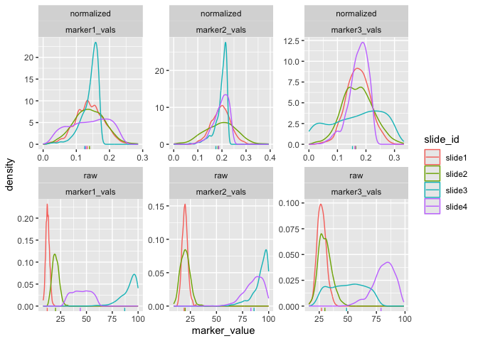
We can also visualize the results of the Otsu misclassification analysis stratified by slide and marker:
plot_mx_discordance(mx_otsu)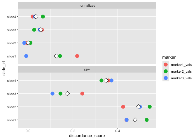
run_reduce_umap()We can also use the UMAP algorithm to reduce the dimensions of our
markers in the dataset as follows, using the metadata_col
parameter for later (e.g., similar to a tissue type in practice with
multiplexed data):
mx_umap = run_reduce_umap(mx_otsu,
                        table="both",
                        marker_list = c("marker1_vals","marker2_vals","marker3_vals"),
                        downsample_pct = 0.8,
                        metadata_col = "metadata1_vals")
We can further visualize the results of the UMAP dimension reduction as follows:
plot_mx_umap(mx_umap,metadata_col = "metadata1_vals")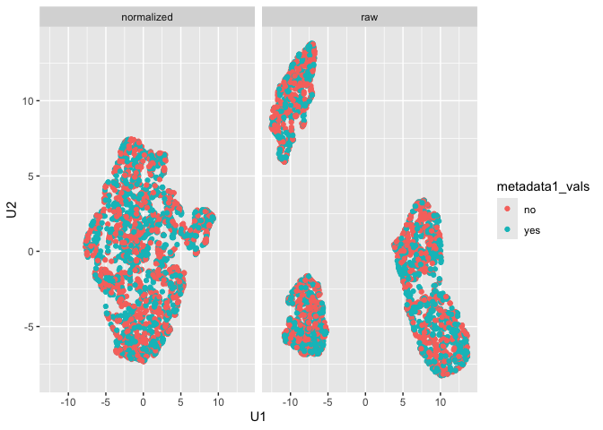
Note that since the sample data is simulated, we don’t see separation
of the groups like we would expect with biological samples that have
some underlying correlation. What we can observe, however, is the
separation of slides in the raw data and subsequent mixing
of these slides in the normalized data:
plot_mx_umap(mx_umap,metadata_col = "slide_id")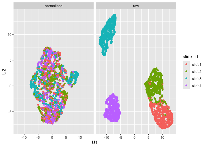
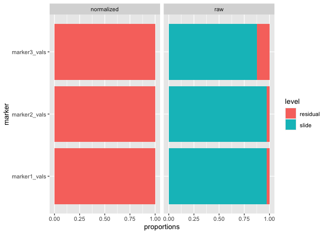
run_var_proportions()We can also leverage lmer() from the lme4
package to perform random effect modeling on the data to determine how
much variance is present at the slide level, as follows:
mx_var = run_var_proportions(mx_umap,
                             table="both",
                             metadata_cols = "metadata1_vals")
And we can use summary() to capture the following
attributes for the mx_dataset object:
summary(mx_var)
#> Call:
#> `mx_dataset` object with 4 slide(s), 3 marker column(s), and 1 metadata column(s)
#>
#> Normalization:
#> Data normalized with transformation=`log10_mean_divide` and method=`None`
#>
#> Anderson-Darling tests:
#>       table mean_test_statistic mean_std_test_statistic mean_p_value
#>  normalized              34.303                  23.911            0
#>         raw              26.656                  18.070            0
#>
#> Threshold discordance scores:
#>       table mean_discordance sd_discordance
#>  normalized            0.054          0.071
#>         raw            0.373          0.141
#>
#> Clustering consistency (UMAP):
#>       table adj_rand_index cohens_kappa
#>  normalized          0.045       -0.054
#>         raw          0.884        0.297
#>
#> Variance proportions (slide-level):
#>       table  mean    sd
#>  normalized 0.001 0.001
#>         raw 0.940 0.055
And we can also visualize the results of the variance proportions after normalization:
plot_mx_proportions(mx_var)