![]()
We implement a surrogate modeling algorithm to guide simulation-based sample size planning. The method is described in detail in a recent paper (Zimmer & Debelak, 2023, https://doi.org/10.1037/met0000611). It supports multiple study design parameters and optimization with respect to a cost function. It can find optimal designs that correspond to a desired statistical power or that fulfill a cost constraint.
Below is a toy example of how to use the package. More in-depth resources are:
You can install the CRAN version using:
install.packages("mlpwr")Or, you can install the development version of mlpwr from GitHub with:
# install.packages("devtools")
devtools::install_github("flxzimmer/mlpwr")This is a basic demonstration to the mlpwr package by going through a toy example. We want to obtain the sample size necessary for a mean comparison using an one-sample t-test.
The package can be loaded via
library(mlpwr)A simulation function (simfun) is a function to generate artificial data and subsequently perform an hypothesis test.
A simple function simulates a group mean comparison with a t-test. The input is a sample size n and the output is either TRUE or FALSE depending on the significance of the hypothesis test.
simfun_ttest <- function(N) {
    # Generate a data set
    dat <- rnorm(n = N, mean = 0.3)
    # Test the hypothesis
    res <- t.test(dat)
    res$p.value < 0.01
}
We can test the data generating function as follows for the sample sizes 30 and 400.
simfun_ttest(30)
#> [1] FALSE
simfun_ttest(400)
#> [1] TRUEThe find.design functions can be used to find an appropriate sample size given a power level that should be surpassed.
The central arguments to be specified are the following:
simfun: The data generating function as defined above.
boundaries: The lower and upper bound to search within, e.g. a sample size between 50 and 200.
power: The desired power of the design.
evaluations: The number of evaluations of the simfun
Once a termination criterion is met (e.g. the number of permissible simfun evaluation specified with evaluations), the algorithm is terminated.
We can perform the search with the above arguments in use.
ds <- find.design(simfun = simfun_ttest, boundaries = c(100,
    300), power = 0.95, evaluations = 4000)
#>  Updates: 1, Evaluations: 1000, Time: 0.1 Updates: 2, Evaluations: 1200, Time: 0.2 Updates: 3, Evaluations: 1400, Time: 0.2 Updates: 4, Evaluations: 1600, Time: 0.3 Updates: 5, Evaluations: 1800, Time: 0.3 Updates: 6, Evaluations: 2000, Time: 0.3 Updates: 7, Evaluations: 2200, Time: 0.4 Updates: 8, Evaluations: 2400, Time: 0.4 Updates: 9, Evaluations: 2600, Time: 0.5 Updates: 10, Evaluations: 2800, Time: 0.5 Updates: 11, Evaluations: 3000, Time: 0.6 Updates: 12, Evaluations: 3200, Time: 0.6 Updates: 13, Evaluations: 3400, Time: 0.6 Updates: 14, Evaluations: 3600, Time: 0.7 Updates: 15, Evaluations: 3800, Time: 0.7 Updates: 16, Evaluations: 4000, Time: 0.8
While it is running, the function gives us some updates regarding the number of updates performed, the time used, and the number of evaluations.
We can get an overview of the results via summary.
summary(ds)
#>
#> Call:
#> find.design(simfun = simfun_ttest, boundaries = c(100, 300),
#>     power = 0.95, evaluations = 4000)
#>
#> Design: N = 201
#>
#> Power: 0.95064,  SE: 0.00379
#> Evaluations: 4000,  Time: 0.86,  Updates: 16
#> Surrogate: Logistic regression
The results indicate that a sample size of 201 is suitable. It shows the predicted power for this sample size, as well as an estimate of its uncertainty (SE). The summary additionally reports the number of simulation function evaluations, the time until termination, and the number of surrogate model updates. The details of the surrogate modeling algorithm are described in our paper.
Also, we can plot the fitted relationship between sample size and power. The black dots show us the simulated data. The gray ribbon indicates the uncertainty of the power at the respective sample sizes.
plot(ds)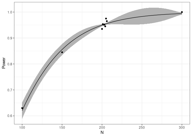
Some templates for simulation functions can be found in the
simulation_functions vignette. It can be accessed at https://github.com/flxzimmer/mlpwr/blob/master/vignettes/simulation_functions.Rmd.