
![]()
This package provides fast implementations of kernel estimators for the copula density. Due to its several plotting options it is particularly useful for the exploratory analysis of dependence structures. It can be further used for flexible nonparametric estimation of copula densities and resampling.
For detailed documentation, see the package vignette and the API documentation.
You can install:
install.packages("kdecopula")devtools::install_github("tnagler/kdecopula")The package provides the following functions:
kdecop: Kernel estimation of a copula density. By
default, estimation method and bandwidth are selected automatically.
Returns an object of class kdecopula.
dkdecop: Evaluates the density of a
kdecopula object.
pkdecop: Evaluates the distribution function of a
kdecopula object.
rkdecop: Simulates synthetic data from a
kdecopula object.
Methods for class kdecopula:
plot, contour: Surface and contour
plots of the density estimate.
print, summary: Displays further
information about the density estimate.
logLik, AIC, BIC: Extracts
fit statistics.
See the API documentation for more details on arguments and options.
Below, we demonstrate the main capabilities of the
kdecopula package. All user-level functions will be
introduced with small examples.
Let’s consider some variables of the Wiscon diagnostic breast cancer data included in this package. The data are transformed to pseudo-observations of the copula by the empirical probability integral/rank transform:
library(kdecopula)
data(wdbc)  # load data
u <- apply(wdbc[, c(2, 8)], 2, rank) / (nrow(wdbc) + 1)  # empirical PIT
plot(u)  # scatter plot
We see that the data are slightly asymmetric w.r.t. both diagonals. Common parametric copula models are usually not flexible enough to reflect this. Let’s see how a kernel estimator does.
We start by estimating the copula density with the
kdecop function. There is a number of options for the
smoothing parameterization, estimation method and evaluation grid, but
it is only required to provide a data-matrix.
kde.fit <- kdecop(u)  # kernel estimation (bandwidth selected automatically)
summary(kde.fit)
#> Kernel copula density estimate (tau = 0.47)
#> ------------------------------
#> Variables:    mean radius -- mean concavity
#> Observations: 569
#> Method:       Transformation local likelihood, log-quadratic (nearest-neighbor, 'TLL2nn')
#> Bandwidth:    alpha = 0.3519647
#>               B = matrix(c(0.71, -0.7, 0.7, 0.71), 2, 2)
#> ---
#> logLik: 201.66    AIC: -367.45    cAIC: -366.21    BIC: -289.53
#> Effective number of parameters: 17.94
The output of the function kdecop is an object of class
kdecopula that contains all information collected during
the estimation process and summary statistics such as AIC or
the effective number of parameters/degrees of freedom. These
can also be accessed directly, e.g.
logLik(kde.fit)
#> 'log Lik.' 201.6617 (df=17.93711)
AIC(kde.fit)
#> [1] -367.4491The most interesting part for most people is probably to make
exploratory plots. The class kdecopula has its own generic
for plotting. In general, there are two possible types of plots:
contour and surface (or perspective) plots.
Additionally, the margins argument allows to choose between
plots of the original copula density and a meta-copula density with
standard normal margins (default for type = contour).
plot(kde.fit)
contour(kde.fit)
contour(kde.fit, margins = "unif")
You can also pass further arguments to the ... argument
to refine the aesthetics. The arguments are forwaded to
lattice::wireframe or graphics::contour,
respectively.
plot(kde.fit,
     zlim = c(0, 10),  # z-axis limits
     screen = list(x = -75, z = 45),  # rotate screen
     xlab = list(rot = 25),  # labels can be rotated as well
ylab = list(label = "other label", rot = -25)) 
contour(kde.fit, col = terrain.colors(30), levels = seq(0, 0.3, by = 0.01))
kdecopula objectThe density and cdf can be computed easily:
dkdecop(c(0.1, 0.2), kde.fit)  # estimated copula density
#> [1] 1.627867
pkdecop(cbind(c(0.1, 0.9), c(0.1, 0.9)), kde.fit) # corresponding copula cdf
#> [1] 0.03164354 0.85004895
Furthermore, we can simulate synthetic data from the estimated density:
unew <- rkdecop(655, kde.fit)
plot(unew)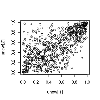
We see that the asymmetries observed in the data are adequately reflected by the estimated model.
Gijbels, I. and Mielniczuk, J. (1990). Estimating the density of a copula function. Communications in Statistics - Theory and Methods, 19(2):445-464.
Charpentier, A., Fermanian, J.-D., and Scaillet, O. (2006). The estimation of copulas: Theory and practice. In Rank, J., editor, Copulas: From theory to application in finance. Risk Books.
Geenens, G., Charpentier, A., and Paindaveine, D. (2014). Probit transformation for nonparametric kernel estimation of the copula density. arXiv:1404.4414 (stat.ME).
Nagler, T. (2014). Kernel Methods for Vine Copula Estimation. Master’s Thesis, Technische Universität München
Wen, K. and Wu, X. (2018). Transformation-Kernel Estimation of Copula Densities. Journal of Business & Economic Statistics, 38(1), 148–164.