![]()
![]()
![]()
The {fHMM} R package allows for the detection and
characterization of financial market regimes in time series data by
applying hidden Markov Models (HMMs). The vignettes outline the
package functionality and the model formulation.
For a reference on the method, see:
Oelschläger, L., and Adam, T. 2021. “Detecting Bearish and Bullish Markets in Financial Time Series Using Hierarchical Hidden Markov Models.” Statistical Modelling. https://doi.org/10.1177/1471082X211034048
A user guide is provided by the accompanying software paper:
Oelschläger, L., Adam, T., and Michels, R. 2024. “fHMM: Hidden Markov Models for Financial Time Series in R”. Journal of Statistical Software. https://doi.org/10.18637/jss.v109.i09
Below, we illustrate an application to the German stock index DAX. We also show how to use the package to simulate HMM data, compute the model likelihood, and decode the hidden states using the Viterbi algorithm.
You can install the released package version from CRAN with:
install.packages("fHMM")We are open to contributions and would appreciate your input:
If you encounter any issues, please submit bug reports as issues.
If you have any ideas for new features, please submit them as feature requests.
If you would like to add extensions to the package, please fork
the master branch and submit a merge request.
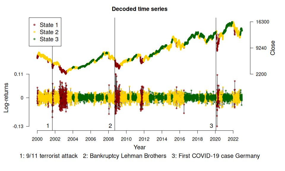
We fit a 3-state HMM with state-dependent t-distributions to the DAX log-returns from 2000 to 2022. The states can be interpreted as proxies for bearish (green below) and bullish markets (red) and an “in-between” market state (yellow).
library("fHMM")The package has a build-in function to download financial data from Yahoo Finance:
dax <- download_data(symbol = "^GDAXI")We first need to define the model:
controls <- set_controls(
  states      = 3,
  sdds        = "t",
  file        = dax,
  date_column = "Date",
  data_column = "Close",
  logreturns  = TRUE,
  from        = "2000-01-01",
  to          = "2022-12-31"
)
The function prepare_data() then prepares the data for
estimation:
data <- prepare_data(controls)The summary() method gives an overview:
summary(data)
#> Summary of fHMM empirical data
#> * number of observations: 5882
#> * data source: data.frame
#> * date column: Date
#> * log returns: TRUE
We fit the model and subsequently decode the hidden states and compute (pseudo-) residuals:
model <- fit_model(data)
model <- decode_states(model)
model <- compute_residuals(model)
The summary() method gives an overview of the model
fit:
summary(model)
#> Summary of fHMM model
#>
#>   simulated hierarchy       LL       AIC       BIC
#> 1     FALSE     FALSE 17650.02 -35270.05 -35169.85
#>
#> State-dependent distributions:
#> t()
#>
#> Estimates:
#>                   lb   estimate        ub
#> Gamma_2.1  2.754e-03  5.024e-03 9.110e-03
#> Gamma_3.1  2.808e-16  2.781e-16 2.739e-16
#> Gamma_1.2  1.006e-02  1.839e-02 3.338e-02
#> Gamma_3.2  1.514e-02  2.446e-02 3.927e-02
#> Gamma_1.3  5.596e-17  5.549e-17 5.464e-17
#> Gamma_2.3  1.196e-02  1.898e-02 2.993e-02
#> mu_1      -3.862e-03 -1.793e-03 2.754e-04
#> mu_2      -7.994e-04 -2.649e-04 2.696e-04
#> mu_3       9.642e-04  1.272e-03 1.579e-03
#> sigma_1    2.354e-02  2.586e-02 2.840e-02
#> sigma_2    1.225e-02  1.300e-02 1.380e-02
#> sigma_3    5.390e-03  5.833e-03 6.312e-03
#> df_1       5.550e+00  1.084e+01 2.116e+01
#> df_2       6.785e+00  4.866e+01 3.489e+02
#> df_3       3.973e+00  5.248e+00 6.934e+00
#>
#> States:
#> decoded
#>    1    2    3
#>  704 2926 2252
#>
#> Residuals:
#>      Min.   1st Qu.    Median      Mean   3rd Qu.      Max.
#> -3.517900 -0.664018  0.012170 -0.003262  0.673180  3.693568
Having estimated the model, we can visualize the state-dependent distributions and the decoded time series:
events <- fHMM_events(
  list(dates = c("2001-09-11", "2008-09-15", "2020-01-27"),
       labels = c("9/11 terrorist attack", "Bankruptcy Lehman Brothers", "First COVID-19 case Germany"))
)
plot(model, plot_type = c("sdds","ts"), events = events)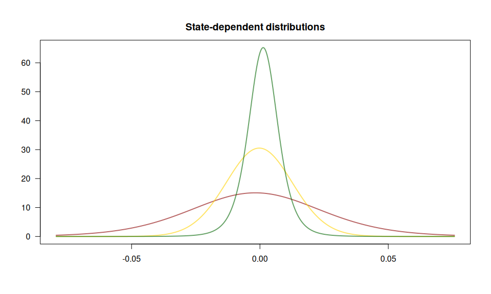
The (pseudo-) residuals help to evaluate the model fit:
plot(model, plot_type = "pr")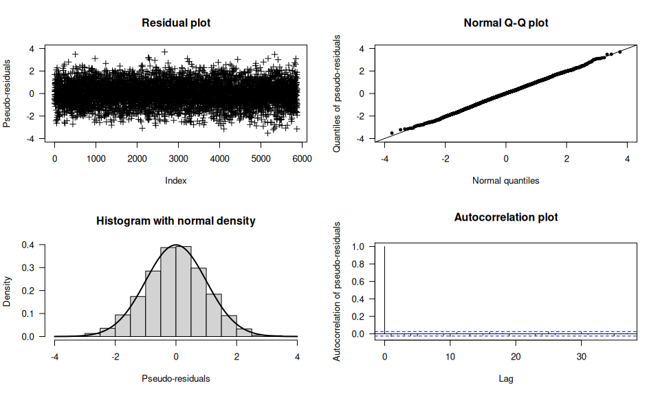
The {fHMM} package supports data simulation from an HMM
and access to the model likelihood function for model fitting and the
Viterbi algorithm for state decoding.
controls <- set_controls(
  states  = 2,
  sdds    = "gamma",
  horizon = 1000
)fHMM_parameters()
function (unspecified parameters would be set at random).par <- fHMM_parameters(
controls = controls,
Gamma = matrix(c(0.95, 0.05, 0.05, 0.95), 2, 2),
mu = c(1, 3),
sigma = c(1, 3)
)simulate_hmm() function.sim <- simulate_hmm(
controls = controls,
true_parameters = par
)
plot(sim$data, col = sim$markov_chain, type = "b")
ll_hmm() is evaluated at
the identified and unconstrained parameter values, they can be derived
via the par2parUncon() function.(parUncon <- par2parUncon(par, controls))
#> gammasUncon_21 gammasUncon_12 muUncon_1 muUncon_2 sigmaUncon_1
#> -2.944439 -2.944439 0.000000 1.098612 0.000000
#> sigmaUncon_2
#> 1.098612
#> attr(,"class")
#> [1] "parUncon" "numeric"Note that this transformation takes care of the restrictions, that
Gamma must be a transition probability matrix (which we can
ensure via the logit link) and that mu and
sigma must be positive (an assumption for the Gamma
distribution, which we can ensure via the exponential link).
ll_hmm(parUncon, sim$data, controls)
#> [1] -1620.515ll_hmm(parUncon, sim$data, controls, negative = TRUE)
#> [1] 1620.515ll_hmm() over parUncon
(or rather minimize the negative log-likelihood).optimization <- nlm(
f = ll_hmm, p = parUncon, observations = sim$data, controls = controls, negative = TRUE
)
(estimate <- optimization$estimate)
#> [1] -3.46338992 -3.44065582 0.05999848 1.06452907 0.11517811 1.07946252parUncon2par()
function. The state-labeling is not identified.class(estimate) <- "parUncon"
estimate <- parUncon2par(estimate, controls)
par$Gamma
#> state_1 state_2
#> state_1 0.95 0.05
#> state_2 0.05 0.95estimate$Gamma
#> state_1 state_2
#> state_1 0.96895125 0.03104875
#> state_2 0.03037204 0.96962796
par$mu
#> muCon_1 muCon_2
#> 1 3estimate$mu
#> muCon_1 muCon_2
#> 1.061835 2.899473
par$sigma
#> sigmaCon_1 sigmaCon_2
#> 1 3estimate$sigma
#> sigmaCon_1 sigmaCon_2
#> 1.122073 2.943097