

![]()
![]()
The bssm R package provides efficient methods for
Bayesian inference of state space models via particle Markov chain Monte
Carlo and importance sampling type weighted MCMC. Currently Gaussian,
Poisson, binomial, negative binomial, and Gamma observation densities
with linear-Gaussian state dynamics, as well as general non-linear
Gaussian models and discretely observed latent diffusion processes are
supported.
For details, see
There are also couple posters and a talk related to IS-correction methodology and bssm package:
The bssm package was originally developed with the
support of Academy of Finland grants 284513, 312605, 311877, and 331817.
Current development is focused on increased usability. For recent
changes, see NEWS file.
If you use the bssm package in publications, please cite
the corresponding R Journal paper:
Jouni Helske and Matti Vihola (2021). “bssm: Bayesian Inference of Non-linear and Non-Gaussian State Space Models in R.” The R Journal (2021) 13:2, pages 578-589. https://journal.r-project.org/archive/2021/RJ-2021-103/index.html
You can install the released version of bssm from CRAN with:
install.packages("bssm")And the development version from GitHub with:
# install.packages("devtools")
devtools::install_github("helske/bssm")
Or from R-universe with
install.packages("bssm", repos = "https://helske.r-universe.dev")Consider the daily air quality measurements in New Your from May to
September 1973, available in the datasets package. Let’s
try to predict the missing ozone levels by simple linear-Gaussian local
linear trend model with temperature and wind as explanatory variables
(missing response variables are handled naturally in the state space
modelling framework, however no missing values in covariates are
normally allowed);
library("bssm")
#> Warning: package 'bssm' was built under R version 4.3.1
#>
#> Attaching package: 'bssm'
#> The following object is masked from 'package:base':
#>
#>     gamma
library("dplyr")
#>
#> Attaching package: 'dplyr'
#> The following objects are masked from 'package:stats':
#>
#>     filter, lag
#> The following objects are masked from 'package:base':
#>
#>     intersect, setdiff, setequal, union
library("ggplot2")
#> Warning: package 'ggplot2' was built under R version 4.3.1
set.seed(1)

data("airquality", package = "datasets")

# Covariates as matrix. For complex cases, check out as_bssm function
xreg <- airquality |> select(Wind, Temp) |> as.matrix()

model <- bsm_lg(airquality$Ozone,
  xreg = xreg,
  # Define priors for hyperparameters (i.e. not the states), see ?bssm_prior
  # Initial value followed by parameters of the prior distribution
  beta = normal_prior(rep(0, ncol(xreg)), 0, 1),
  sd_y = gamma_prior(1, 2, 0.01),
  sd_level = gamma_prior(1, 2, 0.01),
  sd_slope = gamma_prior(1, 2, 0.01))

fit <- run_mcmc(model, iter = 20000, burnin = 5000)
fit
#>
#> Call:
#> run_mcmc.lineargaussian(model = model, iter = 20000, burnin = 5000)
#>
#> Iterations = 5001:20000
#> Thinning interval = 1
#> Length of the final jump chain = 3593
#>
#> Acceptance rate after the burn-in period:  0.239
#>
#> Summary for theta:
#>
#>  variable       Mean          SE        SD        2.5%     97.5% ESS
#>      Temp  1.0265846 0.007497538 0.2064343  0.60226671  1.400436 758
#>      Wind -2.5183269 0.020978488 0.5764833 -3.68987992 -1.327578 755
#>  sd_level  6.3731836 0.113153715 2.8013937  1.52958636 12.403961 613
#>  sd_slope  0.3388712 0.010355574 0.2833955  0.04210885  1.070284 749
#>      sd_y 20.8618647 0.068145131 1.9369381 17.08728231 24.722309 808
#>
#> Summary for alpha_154:
#>
#>  variable time        Mean         SE        SD       2.5%     97.5%  ESS
#>     level  154 -28.3163054 0.69650977 20.132341 -69.271049 11.797133  835
#>     slope  154  -0.3740463 0.03683278  1.685733  -4.065499  2.830134 2094
#>
#> Run time:
#>    user  system elapsed
#>    0.57    0.02    0.63

obs <- data.frame(Time = 1:nrow(airquality),
  Ozone = airquality$Ozone) |> filter(!is.na(Ozone))

pred <- fitted(fit, model)
pred |>
  ggplot(aes(x = Time, y = Mean)) +
  geom_ribbon(aes(ymin = `2.5%`, ymax = `97.5%`),
    alpha = 0.5, fill = "steelblue") +
  geom_line() +
  geom_point(data = obs,
    aes(x = Time, y = Ozone), colour = "Tomato") +
  theme_bw()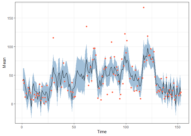
Same model but now assuming observations are from Gamma distribution:
model2 <- bsm_ng(airquality$Ozone,
  xreg = xreg,
  beta = normal(rep(0, ncol(xreg)), 0, 1),
  distribution = "gamma",
  phi = gamma_prior(1, 2, 0.01),
  sd_level = gamma_prior(1, 2, 0.1),
  sd_slope = gamma_prior(1, 2, 0.1))

fit2 <- run_mcmc(model2, iter = 20000, burnin = 5000, particles = 10)
fit2
#>
#> Call:
#> run_mcmc.nongaussian(model = model2, iter = 20000, particles = 10,
#>     burnin = 5000)
#>
#> Iterations = 5001:20000
#> Thinning interval = 1
#> Length of the final jump chain = 3858
#>
#> Acceptance rate after the burn-in period:  0.257
#>
#> Summary for theta:
#>
#>  variable         Mean           SE          SD          2.5%       97.5%  ESS
#>      Temp  0.052808820 0.0002404538 0.008701489  0.0353736458  0.06992423 1310
#>      Wind -0.057351094 0.0004338213 0.015411504 -0.0873384757 -0.02700112 1262
#>       phi  4.006977632 0.0159088062 0.536273508  3.0263444882  5.15527365 1136
#>  sd_level  0.057158663 0.0020138200 0.035366227  0.0083794202  0.14651419  308
#>  sd_slope  0.003894013 0.0001752319 0.003654978  0.0004250207  0.01374575  435
#>         SE_IS ESS_IS
#>  7.128104e-05  14485
#>  1.263047e-04  13905
#>  4.411840e-03  14611
#>  2.927386e-04  10591
#>  3.031489e-05   7766
#>
#> Summary for alpha_154:
#>
#>  variable time         Mean           SE         SD        2.5%      97.5%  ESS
#>     level  154 -0.200656509 0.0201721601 0.73134471 -1.62501396 1.24522802 1314
#>     slope  154 -0.002689176 0.0005121944 0.02289051 -0.04650504 0.04724173 1997
#>        SE_IS ESS_IS
#>  0.005987284   9458
#>  0.000191620   6448
#>
#> Run time:
#>    user  system elapsed
#>    7.50    0.01    7.71
Comparison:
pred2 <- fitted(fit2, model2)

bind_rows(list(Gaussian = pred, Gamma = pred2), .id = "Model") |>
  ggplot(aes(x = Time, y = Mean)) +
  geom_ribbon(aes(ymin = `2.5%`, ymax = `97.5%`, fill = Model),
    alpha = 0.25) +
  geom_line(aes(colour = Model)) +
  geom_point(data = obs,
    aes(x = Time, y = Ozone)) +
  theme_bw()
Now let’s assume that we also want to use the solar radiation variable as predictor for ozone. As it contains few missing values, we cannot use it directly. As the number of missing time points is very small, simple imputation would likely be acceptable, but let’s consider more another approach. For simplicity, the slope terms of the previous models are now omitted, and we focus on the Gaussian case. Let \(\mu_t\) be the true solar radiation at time \(t\). Now for ozone \(O_t\) we assume following model:
\(O_t = D_t + \alpha_t + \beta_S \mu_t +
\sigma_\epsilon \epsilon_t\)
\(\alpha_{t+1} = \alpha_t +
\sigma_\eta\eta_t\)
\(\alpha_1 \sim N(0,
100^2\textrm{I})\),
wheere \(D_t = \beta X_t\) contains
regression terms related to wind and temperature, \(\alpha_t\) is the time varying intercept
term, and \(\beta_S\) is the effect of
solar radiation \(\mu_t\).
Now for the observed solar radiation \(S_t\) we assume
\(S_t = \mu_t\)
\(\mu_{t+1} = \mu_t +
\sigma_\xi\xi_t,\)
\(\mu_1 \sim N(0, 100^2)\),
i.e. we assume as simple random walk for the \(\mu\) which we observe without error or not
at all (there is no error term in the observation equation \(S_t=\mu_t\)).
We combine these two models as a bivariate Gaussian model with
ssm_mlg:
# predictors (not including solar radiation) for ozone
xreg <- airquality |> select(Wind, Temp) |> as.matrix()

# Function which outputs new model components given the parameter vector theta
update_fn <- function(theta) {
  D <- rbind(t(xreg %*% theta[1:2]), 1)
  Z <- matrix(c(1, 0, theta[3], 1), 2, 2)
  R <- diag(exp(theta[4:5]))
  H <- diag(c(exp(theta[6]), 0))
  # add third dimension so we have p x n x 1, p x m x 1, p x p x 1 arrays
  dim(Z)[3] <- dim(R)[3] <- dim(H)[3] <- 1
  list(D = D, Z = Z, R = R, H = H)
}

# Function for log-prior density
prior_fn <- function(theta) {
  sum(dnorm(theta[1:3], 0, 10, log = TRUE)) +
    sum(dgamma(exp(theta[4:6]), 2, 0.01, log = TRUE)) +
    sum(theta[4:6]) # log-jacobian
}

init_theta <- c(0, 0, 0, log(50), log(5), log(20))
comps <- update_fn(init_theta)

model <- ssm_mlg(y = cbind(Ozone = airquality$Ozone, Solar = airquality$Solar.R),
  Z = comps$Z, D = comps$D, H = comps$H, T = diag(2), R = comps$R,
  a1 = rep(0, 2), P1 = diag(100, 2), init_theta = init_theta,
  state_names = c("alpha", "mu"), update_fn = update_fn,
  prior_fn = prior_fn)

fit <- run_mcmc(model, iter = 60000, burnin = 10000)
fit
#>
#> Call:
#> run_mcmc.lineargaussian(model = model, iter = 60000, burnin = 10000)
#>
#> Iterations = 10001:60000
#> Thinning interval = 1
#> Length of the final jump chain = 12234
#>
#> Acceptance rate after the burn-in period:  0.245
#>
#> Summary for theta:
#>
#>  variable        Mean           SE         SD       2.5%      97.5%  ESS
#>   theta_1 -3.89121114 0.0233827004 0.58715113 -5.0085134 -2.6915137  631
#>   theta_2  0.98712126 0.0051506907 0.18819758  0.5917823  1.3475147 1335
#>   theta_3  0.06324657 0.0004672314 0.02417334  0.0141425  0.1100184 2677
#>   theta_4  0.82577262 0.0165661049 0.67134723 -0.6840637  1.9160168 1642
#>   theta_5  4.75567621 0.0010887250 0.05858454  4.6446809  4.8704036 2895
#>   theta_6  3.05462451 0.0014803971 0.07640392  2.9032635  3.2028023 2664
#>
#> Summary for alpha_154:
#>
#>  variable time      Mean        SE        SD       2.5%     97.5%  ESS
#>     alpha  154 -16.44435 0.3659912  14.99708 -46.321645  13.01863 1679
#>        mu  154 223.60490 1.3409568 116.49063  -6.206301 453.18554 7546
#>
#> Run time:
#>    user  system elapsed
#>    7.41    0.11    7.83
Draw predictions:
pred <- fitted(fit, model)

obs <- data.frame(Time = 1:nrow(airquality),
  Solar = airquality$Solar.R) |> filter(!is.na(Solar))

pred |> filter(Variable == "Solar") |>
  ggplot(aes(x = Time, y = Mean)) +
  geom_ribbon(aes(ymin = `2.5%`, ymax = `97.5%`),
    alpha = 0.5, fill = "steelblue") +
  geom_line() +
  geom_point(data = obs,
    aes(x = Time, y = Solar), colour = "Tomato") +
  theme_bw()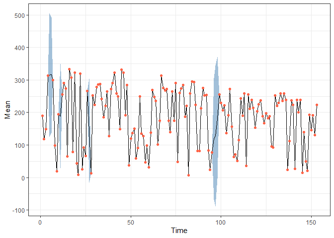
obs <- data.frame(Time = 1:nrow(airquality),
  Ozone = airquality$Ozone) |> filter(!is.na(Ozone))

pred |> filter(Variable == "Ozone") |>
  ggplot(aes(x = Time, y = Mean)) +
  geom_ribbon(aes(ymin = `2.5%`, ymax = `97.5%`),
    alpha = 0.5, fill = "steelblue") +
  geom_line() +
  geom_point(data = obs,
    aes(x = Time, y = Ozone), colour = "Tomato") +
  theme_bw()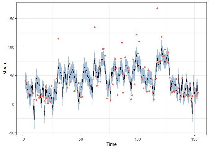
See more examples in the paper, vignettes, and in the docs.