
The goal of bltm is to fit Bayesian Latent Threshold Models using R. The model in the AR(1) form is defined by these equations:
[ \[\begin{aligned} y_{it} &= \sum_{j=1}^J x_{ijt} b_{ijt} + \varepsilon_{it} \\ b_{ijt} &= \beta_{ijt} \,\mathbb I(|\beta_{ijt}| \geq d_{ij}) \\ \beta_{ij,t+1} &= \mu_{ij} + \phi_{ij}(\beta_{ijt}-\mu_{ij}) + \eta_{ijt} \end{aligned}\]]
for (i ,, I), (j ,, J) and (t ,, T). These models can be fit separatedly for each (i). The example below fits the model to one single series ((I=1)).
library(tidyverse)
#> ── Attaching packages ───────────────────────────────────────────────────────────────────── tidyverse 1.2.1 ──
#> ✔ ggplot2 3.2.0          ✔ purrr   0.3.2
#> ✔ tibble  2.1.3          ✔ dplyr   0.8.1
#> ✔ tidyr   0.8.3.9000     ✔ stringr 1.4.0
#> ✔ readr   1.3.1          ✔ forcats 0.4.0
#> ── Conflicts ──────────────────────────────────────────────────────────────────────── tidyverse_conflicts() ──
#> ✖ dplyr::filter() masks stats::filter()
#> ✖ dplyr::lag()    masks stats::lag()
devtools::load_all()
#> Loading bltmset.seed(103)
d_sim <- ltm_sim(
ni = 5, ns = 500, nk = 2,
alpha = 0,
vmu = matrix(c(.5,.5), nrow = 2),
mPhi = diag(2) * c(.99, .99),
mSigs = c(.1,.1),
dsig = .15,
vd = matrix(c(.4,.4), nrow = 2)
)
# adding zeroed beta
binder <- array(runif(500)-.5, c(5, 500, 1))
d_sim$mx <- abind::abind(d_sim$mx, binder, along = 3)
d_sim$mb <- cbind(d_sim$mb, 0)result <- ltm_mcmc(d_sim$mx, d_sim$vy, burnin = 100, iter = 500)
# readr::write_rds(result, "data-raw/result.rds", compress = "xz")Iteration: 1 / 600 [ 0%] (Warmup)
Iteration: 60 / 600 [ 10%] (Warmup)
Iteration: 120 / 600 [ 20%] (Sampling)
Iteration: 180 / 600 [ 30%] (Sampling)
Iteration: 240 / 600 [ 40%] (Sampling)
Iteration: 300 / 600 [ 50%] (Sampling)
Iteration: 360 / 600 [ 60%] (Sampling)
Iteration: 420 / 600 [ 70%] (Sampling)
Iteration: 480 / 600 [ 80%] (Sampling)
Iteration: 540 / 600 [ 90%] (Sampling)
Iteration: 600 / 600 [ 100%] (Sampling)Results after 100 burnin and 500 iterations.
result <- read_rds("data-raw/result.rds")vars_to_analyse <- !str_detect(colnames(result), "beta\\[")
summary_table <- result[,vars_to_analyse] %>%
as.data.frame() %>%
tibble::rowid_to_column() %>%
tidyr::gather(key, val, -rowid) %>%
dplyr::group_by(key) %>%
dplyr::summarise(
median = median(val),
sd = sd(val),
q025 = quantile(val, 0.025),
q975 = quantile(val, 0.975)
)
knitr::kable(summary_table)| key | median | sd | q025 | q975 |
|---|---|---|---|---|
| alpha[1] | 0.0076648 | 0.1781915 | -0.3405058 | 0.3593770 |
| alpha[2] | -0.0054158 | 0.1830903 | -0.3785451 | 0.3289486 |
| alpha[3] | -0.0047880 | 0.1834158 | -0.3854517 | 0.3297607 |
| alpha[4] | -0.0163057 | 0.1746813 | -0.3578320 | 0.2923298 |
| alpha[5] | -0.0016525 | 0.1801260 | -0.3304960 | 0.3382569 |
| d[1] | 0.3293945 | 0.0496160 | 0.2324488 | 0.4076028 |
| d[2] | 0.0150496 | 0.0559342 | 0.0150496 | 0.1553439 |
| d[3] | 0.2701171 | 0.0146839 | 0.2296899 | 0.2701171 |
| mu[1] | 0.5296798 | 0.3416395 | -0.2345459 | 1.0597430 |
| mu[2] | 0.5947912 | 0.2164022 | 0.1596099 | 1.0128513 |
| mu[3] | 0.0665906 | 0.0173249 | 0.0260728 | 0.0945483 |
| phi[1] | 0.9904074 | 0.0050235 | 0.9784768 | 0.9977583 |
| phi[2] | 0.9713490 | 0.0113390 | 0.9458727 | 0.9921012 |
| phi[3] | 0.6437641 | 0.1325909 | 0.3581005 | 0.8528770 |
| sig_eta[1] | 0.0731782 | 0.0083558 | 0.0561148 | 0.0888805 |
| sig_eta[2] | 0.1222165 | 0.0138444 | 0.0921127 | 0.1494326 |
| sig_eta[3] | 0.0623744 | 0.0100680 | 0.0486990 | 0.0867437 |
| sig[1] | 0.1760752 | 0.0045631 | 0.1677408 | 0.1878592 |
bayesplot::mcmc_trace(result, regex_pars = "mu\\[[12]") +
  theme_bw()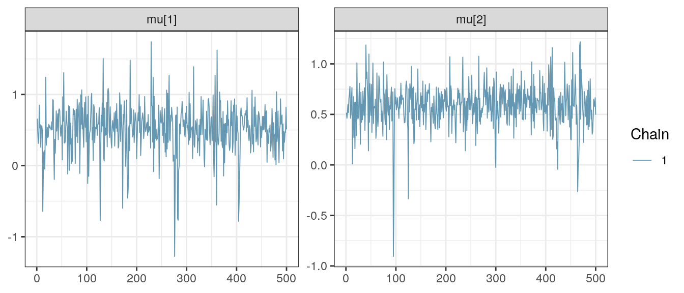
# check this function inside demo/ folder
source("demo/plot_betas.R")
plot_betas(result, 1:3, real_values = d_sim) +
  facet_wrap(~factor(p), ncol = 2) +
  theme_bw()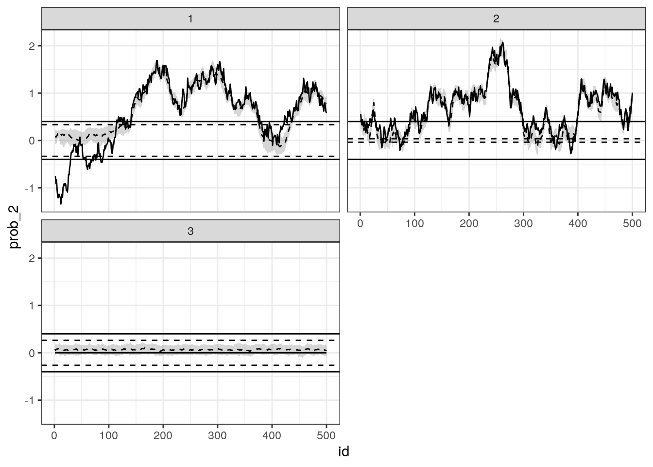
[y_i = T {t=1} y{it}]
[^{*}_{} = ,]
where
[a^*i={t=1}^{T}{k=1}^{K}x{itk}_{tk}]
Generate using
[^{*} N(_{}^{}, ^{2}),]
where (^{*2}) is the posterior sample of ()
The difference between the paper and the code is that it checks if some of the () should be replaced by zero. Actually, it is not a difference; the appendix is just a little obscure in this passage.
First, we calculate (M_t) and (m_t) (depending on (t)), then we generate candidates for (_t) and their log-densities using the normal distribution.
We then recalculate (M_t) and (m_t), replacing some of (x_t)s entries by zero, depending on a condition based on the threshold and the values of (). Finally, we obtain the log-density of the previously calculated (m_t) using these new parameters. This is the MH step where we draw a candidate from a (auxiliary) posterior distribution of non-threshold model. When we decide to accept the candidate, we compute the posterior distribution of the auxiliary posterior distribution and the true posterior distribution (of the threshold model). For the latter, we need to replace some of (x_t)’s entries by zero depending on a condition based on the threshold and the betas.
It’s important to note that if there aren’t any () to replace by zero, then we should accept the new () with probability one, because the posterior has an analytic formula.
MIT