Behavioral economic demand is gaining in popularity. The motivation
behind beezdemand was to create an alternative tool to
conduct these analyses. This package is not necessarily meant to be a
replacement for other softwares; rather, it is meant to serve as an
additional tool in the behavioral economist’s toolbox. It is meant for
researchers to conduct behavioral economic (be) demand the easy (ez)
way.
Currently, this version (0.1.0) is the first minor release and is stable. I encourage you to use it but be aware that, as with any software release, there might be (unknown) bugs present. I’ve tried hard to make this version usable while including the core functionality (described more below). However, if you find issues or would like to contribute, please open an issue on my GitHub page or email me.
The latest stable version of beezdemand (currently
v.0.1.0) can be found on CRAN and
installed using the following command. The first time you install the
package, you may be asked to select a CRAN mirror. Simply select the
mirror geographically closest to you.
install.packages("beezdemand")

library(beezdemand)To install a stable release directly from GitHub, first
install and load the devtools package. Then, use
install_github to install the package and associated
vignette. You don’t need to download anything directly from GitHub, as you
should use the following instructions:
install.packages("devtools")

devtools::install_github("brentkaplan/beezdemand", build_vignettes = TRUE)

library(beezdemand)To install the development version of the package, specify the
development branch in install_github:
devtools::install_github("brentkaplan/beezdemand@develop")An example dataset of responses on an Alcohol Purchase Task is
provided. This object is called apt and is located within
the beezdemand package. These data are a subset of from the
paper by Kaplan
& Reed (2018). Participants (id) reported the number of
alcoholic drinks (y) they would be willing to purchase and consume at
various prices (x; USD). Note the format of the data, which is called
“long format”. Long format data are data structured such that repeated
observations are stacked in multiple rows, rather than across columns.
First, take a look at an extract of the dataset apt, where
I’ve subsetted rows 1 through 10 and 17 through 26:
| id | x | y | |
|---|---|---|---|
| 1 | 19 | 0.0 | 10 |
| 2 | 19 | 0.5 | 10 |
| 3 | 19 | 1.0 | 10 |
| 4 | 19 | 1.5 | 8 |
| 5 | 19 | 2.0 | 8 |
| 6 | 19 | 2.5 | 8 |
| 7 | 19 | 3.0 | 7 |
| 8 | 19 | 4.0 | 7 |
| 9 | 19 | 5.0 | 7 |
| 10 | 19 | 6.0 | 6 |
| 17 | 30 | 0.0 | 3 |
| 18 | 30 | 0.5 | 3 |
| 19 | 30 | 1.0 | 3 |
| 20 | 30 | 1.5 | 3 |
| 21 | 30 | 2.0 | 2 |
| 22 | 30 | 2.5 | 2 |
| 23 | 30 | 3.0 | 2 |
| 24 | 30 | 4.0 | 2 |
| 25 | 30 | 5.0 | 2 |
| 26 | 30 | 6.0 | 2 |
The first column contains the row number. The second column contains the id number of the series within the dataset. The third column contains the x values (in this specific dataset, price per drink) and the fourth column contains the associated responses (number of alcoholic drinks purchased at each respective price). There are replicates of id because for each series (or participant), several x values were presented.
Take for example the format of most datasets that would be exported from a data collection software such as Qualtrics or SurveyMonkey or Google Forms:
## the following code takes the apt data, which are in long format, and converts
## to a wide format that might be seen from data collection software
wide <- spread(apt, x, y)
colnames(wide) <- c("id", paste0("price_", seq(1, 16, by = 1)))
knitr::kable(wide[1:5, 1:10])| id | price_1 | price_2 | price_3 | price_4 | price_5 | price_6 | price_7 | price_8 | price_9 |
|---|---|---|---|---|---|---|---|---|---|
| 19 | 10 | 10 | 10 | 8 | 8 | 8 | 7 | 7 | 7 |
| 30 | 3 | 3 | 3 | 3 | 2 | 2 | 2 | 2 | 2 |
| 38 | 4 | 4 | 4 | 4 | 4 | 4 | 4 | 3 | 3 |
| 60 | 10 | 10 | 8 | 8 | 6 | 6 | 5 | 5 | 4 |
| 68 | 10 | 10 | 9 | 9 | 8 | 8 | 7 | 6 | 5 |
A dataset such as this is referred to as “wide format” because each
participant series contains a single row and multiple measurements
within the participant are indicated by the columns. This data format is
fine for some purposes; however, for beezdemand, data are
required to be in “long format” (in the same format as the example data
described earlier). In order to convert to the
long format, some steps will be required.
First, it is helpful to rename the columns to what the prices actually were. For example, for the purposes of our example dataset, price_1 was $0.00 (free), price_2 was $0.50, price_3 was $1.00, and so on.
## make an object to hold what will be the new column names
newcolnames <- c("id", "0", "0.5", "1", "1.50", "2", "2.50", "3",
                 "4", "5", "6", "7", "8", "9", "10", "15", "20")
## current column names
colnames(wide)
[1] "id" "price_1" "price_2" "price_3" "price_4" "price_5"
[7] "price_6" "price_7" "price_8" "price_9" "price_10" "price_11"
[13] "price_12" "price_13" "price_14" "price_15" "price_16"## replace current column names with new column names
colnames(wide) <- newcolnames
## how new data look (first 5 rows only)
knitr::kable(wide[1:5, ])| id | 0 | 0.5 | 1 | 1.50 | 2 | 2.50 | 3 | 4 | 5 | 6 | 7 | 8 | 9 | 10 | 15 | 20 |
|---|---|---|---|---|---|---|---|---|---|---|---|---|---|---|---|---|
| 19 | 10 | 10 | 10 | 8 | 8 | 8 | 7 | 7 | 7 | 6 | 6 | 5 | 5 | 4 | 3 | 2 |
| 30 | 3 | 3 | 3 | 3 | 2 | 2 | 2 | 2 | 2 | 2 | 2 | 2 | 1 | 1 | 1 | 1 |
| 38 | 4 | 4 | 4 | 4 | 4 | 4 | 4 | 3 | 3 | 3 | 3 | 2 | 2 | 2 | 0 | 0 |
| 60 | 10 | 10 | 8 | 8 | 6 | 6 | 5 | 5 | 4 | 4 | 3 | 3 | 2 | 2 | 0 | 0 |
| 68 | 10 | 10 | 9 | 9 | 8 | 8 | 7 | 6 | 5 | 5 | 5 | 4 | 4 | 3 | 0 | 0 |
Now we can convert into a long format using some of the helpful
functions in the tidyverse package (make sure the package
is loaded before trying the commands below).
## using the dataframe 'wide', we specify the key will be 'price', the values
## will be 'consumption', and we will select all columns besides the first ('id')
long <- tidyr::gather(wide, price, consumption, -id)

## we'll sort the rows by id
long <- arrange(long, id)

## view the first 20 rows
knitr::kable(long[1:20, ])| id | price | consumption |
|---|---|---|
| 19 | 0 | 10 |
| 19 | 0.5 | 10 |
| 19 | 1 | 10 |
| 19 | 1.50 | 8 |
| 19 | 2 | 8 |
| 19 | 2.50 | 8 |
| 19 | 3 | 7 |
| 19 | 4 | 7 |
| 19 | 5 | 7 |
| 19 | 6 | 6 |
| 19 | 7 | 6 |
| 19 | 8 | 5 |
| 19 | 9 | 5 |
| 19 | 10 | 4 |
| 19 | 15 | 3 |
| 19 | 20 | 2 |
| 30 | 0 | 3 |
| 30 | 0.5 | 3 |
| 30 | 1 | 3 |
| 30 | 1.50 | 3 |
Two final modifications we will make will be to (1) rename our
columns to what the functions in beezdemand will expect to
see: id, x, and y, and (2) ensure
both x and y are in numeric format.
colnames(long) <- c("id", "x", "y")

long$x <- as.numeric(long$x)
long$y <- as.numeric(long$y)
knitr::kable(head(long))| id | x | y |
|---|---|---|
| 19 | 0.0 | 10 |
| 19 | 0.5 | 10 |
| 19 | 1.0 | 10 |
| 19 | 1.5 | 8 |
| 19 | 2.0 | 8 |
| 19 | 2.5 | 8 |
The dataset is now “tidy” because: (1) each variable forms a column, (2) each observation forms a row, and (3) each type of observational unit forms a table (in this case, our observational unit is the Alcohol Purchase Task data). To learn more about the benefits of tidy data, readers are encouraged to consult Hadley Wikham’s essay on Tidy Data.
Descriptive values of responses at each price can be obtained easily.
The resulting table includes mean, standard deviation, proportion of
zeros, number of NAs, and minimum and maximum values. If
bwplot = TRUE, a box-and-whisker plot is also created and
saved. By default, this location is a folder named “plots” one level up
from the current working directory. The user may additionally specify
the directory that the plot should save into, the type of file (either
"png" or "pdf"), and the filename. Notice the
red crosses indicate the mean. Defaults are shown here:
GetDescriptives(dat = apt, bwplot = FALSE, outdir = "../plots/", device = "png",
                filename = "bwplot")
To actually run the code and generate the file, we will turn
bwplot = TRUE. The function will create a folder one level
higher than the current folder (i.e., the ../ portion) and
save the file, “bwplot.png” in the folder.
GetDescriptives(dat = apt, bwplot = TRUE, outdir = plotdir, device = "png",
                filename = "bwplot")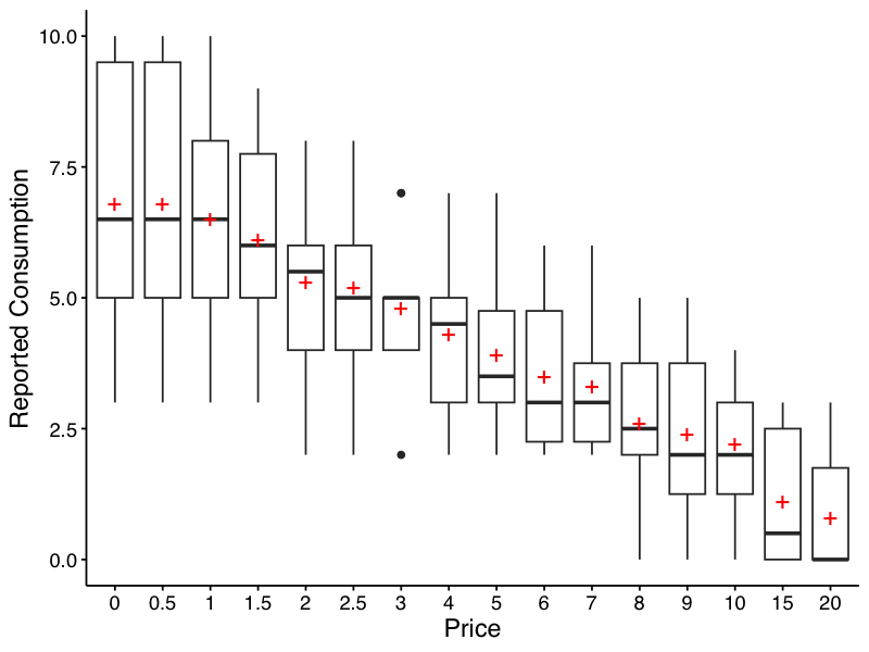
And here is the table that is returned from the function:
| Price | Mean | Median | SD | PropZeros | NAs | Min | Max |
|---|---|---|---|---|---|---|---|
| 0 | 6.8 | 6.5 | 2.62 | 0.0 | 0 | 3 | 10 |
| 0.5 | 6.8 | 6.5 | 2.62 | 0.0 | 0 | 3 | 10 |
| 1 | 6.5 | 6.5 | 2.27 | 0.0 | 0 | 3 | 10 |
| 1.5 | 6.1 | 6.0 | 1.91 | 0.0 | 0 | 3 | 9 |
| 2 | 5.3 | 5.5 | 1.89 | 0.0 | 0 | 2 | 8 |
| 2.5 | 5.2 | 5.0 | 1.87 | 0.0 | 0 | 2 | 8 |
| 3 | 4.8 | 5.0 | 1.48 | 0.0 | 0 | 2 | 7 |
| 4 | 4.3 | 4.5 | 1.57 | 0.0 | 0 | 2 | 7 |
| 5 | 3.9 | 3.5 | 1.45 | 0.0 | 0 | 2 | 7 |
| 6 | 3.5 | 3.0 | 1.43 | 0.0 | 0 | 2 | 6 |
| 7 | 3.3 | 3.0 | 1.34 | 0.0 | 0 | 2 | 6 |
| 8 | 2.6 | 2.5 | 1.51 | 0.1 | 0 | 0 | 5 |
| 9 | 2.4 | 2.0 | 1.58 | 0.1 | 0 | 0 | 5 |
| 10 | 2.2 | 2.0 | 1.32 | 0.1 | 0 | 0 | 4 |
| 15 | 1.1 | 0.5 | 1.37 | 0.5 | 0 | 0 | 3 |
| 20 | 0.8 | 0.0 | 1.14 | 0.6 | 0 | 0 | 3 |
There are certain instances in which data are to be modified before fitting, for example when using an equation that logarithmically transforms y values. The following function can help with modifying data:
nrepl indicates number of replacement 0 values,
either as an integer or "all". If this value is an integer,
n, then the first n 0s will be
replaced.
replnum indicates the number that should replace 0
values
rem0 removes all zeros
remq0e removes y value where x (or price) equals
0
replfree replaces where x (or price) equals 0 with a
specified number
ChangeData(dat = apt, nrepl = 1, replnum = 0.01, rem0 = FALSE, remq0e = FALSE,
replfree = NULL)Using the following function, we can examine the consistency of demand data using Stein et al.’s (2015) alogrithm for identifying unsystematic responses. Default values shown, but they can be customized.
CheckUnsystematic(dat = apt, deltaq = 0.025, bounce = 0.1, reversals = 0, ncons0 = 2)| id | TotalPass | DeltaQ | DeltaQPass | Bounce | BouncePass | Reversals | ReversalsPass | NumPosValues |
|---|---|---|---|---|---|---|---|---|
| 19 | 3 | 0.2112 | Pass | 0 | Pass | 0 | Pass | 16 |
| 30 | 3 | 0.1437 | Pass | 0 | Pass | 0 | Pass | 16 |
| 38 | 3 | 0.7885 | Pass | 0 | Pass | 0 | Pass | 14 |
| 60 | 3 | 0.9089 | Pass | 0 | Pass | 0 | Pass | 14 |
| 68 | 3 | 0.9089 | Pass | 0 | Pass | 0 | Pass | 14 |
Results of the analysis return both empirical and derived measures for use in additional analyses and model specification. Equations include the linear model, exponential model, and exponentiated model. Soon, I will be including the nonlinear mixed effects model, mixed effects versions of the exponential and exponentiated model, and others. However, currently these models are not yet supported.
Empirical measures can be obtained separately on their own:
GetEmpirical(dat = apt)| id | Intensity | BP0 | BP1 | Omaxe | Pmaxe |
|---|---|---|---|---|---|
| 19 | 10 | NA | 20 | 45 | 15 |
| 30 | 3 | NA | 20 | 20 | 20 |
| 38 | 4 | 15 | 10 | 21 | 7 |
| 60 | 10 | 15 | 10 | 24 | 8 |
| 68 | 10 | 15 | 10 | 36 | 9 |
FitCurves() has several important arguments that can be
passed. For the purposes of this document, focus will be on the two
contemporary demand equations.
equation = "hs" is the default but can accept the
character strings "linear", "hs", or
"koff", the latter two of which are the contemporary
equations proposed by Hursh &
Silberberg (2008) and Koffarnus et
al. (2015), respectively.
k can take accept a specific number but by default
will be calculated based on the maximum and minimum y values of the
entire sample and adding .5. Adding this amount was originally proposed
by Steven R. Hursh in an early iteration of a Microsoft Excel
spreadsheet used to calculate demand metrics. This adjustment was
adopted for two reasons. First, when fitting \(Q_0\) as a derived parameter, the value may
exceed the empirically observed intensity value. Thus, a k value
calculated based only on the observed range of data may underestimate
the full fitted range of the curve. Second, we have found that values of
\(\alpha\) (as well as values that rely
on \(\alpha\), i.e. approximate \(P_{max}\)) display greater discrepancies
when smaller values of k are used compared to larger values of k. Other
options include "ind", which will calculate k based on
individual basis, "fit", which will fit k as a free
parameter on an individual basis, "share", which will fit k
as a single shared parameter across all data sets (while fitting
individual \(Q_0\) and \(\alpha\)).
agg = NULL is the default, which means no
aggregation. When agg = "Mean", models are fit to the
averaged data disregarding any error. When agg = "Pooled",
all data are used and clustering within individual is ignored.
detailed = FALSE is the default. This will output a
single dataframe of results, as shown below. When
detailed = TRUE, the output is a 3 element list that
includes (1) dataframe of results, (2) list of nonlinear regression
model objects, (3) list of dataframes containing predicted x and y
values (to be used in subsequent plotting), and (4) list of individual
dataframes used in fitting.
lobound and hibound can accept named
vectors that will be used as lower and upper bounds, respectively during
fitting. If k = "fit", then it should look as follows
(values are nonspecific):
lobound = c("q0" = 0, "k" = 0, "alpha" = 0) and
hibound = c("q0" = 25, "k" = 10, "alpha" = 1). If
k is not being fit as a parameter, then only
"q0" and "alpha" should be used in
bounding.
Note: Fitting with an equation (e.g., "linear",
"hs") that doesn’t work happily with zero consumption
values results in the following. One, a message will appear saying that
zeros are incompatible with the equation. Two, because zeros are removed
prior to finding empirical (i.e., observed) measures, resulting BP0
values will be all NAs (reflective of the data transformations). The
warning message will look as follows:
Warning message:
Zeros found in data not compatible with equation! Dropping zeros!
The simplest use of FitCurves() is shown here, only
needing to specify dat and equation. All other
arguments shown are set to their default values.
FitCurves(dat = apt, equation = "hs", agg = NULL, detailed = FALSE,
          xcol = "x", ycol = "y", idcol = "id", groupcol = NULL)
Which is equivalent to:
FitCurves(dat = apt, equation = "hs")Note that this ouput returns a message
(No k value specified. Defaulting to empirical mean range +.5)
and the aforementioned warning
(Warning message: Zeros found in data not compatible with equation! Dropping zeros!).
With detailed = FALSE, the only output is the dataframe of
results (broken up to show the different types of results). This example
fits the exponential equation proposed by Hursh &
Silberberg (2008):
| id | Intensity | BP0 | BP1 | Omaxe | Pmaxe |
|---|---|---|---|---|---|
| 19 | 10 | NA | 20 | 45 | 15 |
| 30 | 3 | NA | 20 | 20 | 20 |
| 38 | 4 | NA | 10 | 21 | 7 |
| 60 | 10 | NA | 10 | 24 | 8 |
| 68 | 10 | NA | 10 | 36 | 9 |
Empirical Measures
| Equation | Q0d | K | Alpha | R2 |
|---|---|---|---|---|
| hs | 10.475734 | 1.031479 | 0.0046571 | 0.9660008 |
| hs | 2.932406 | 1.031479 | 0.0134557 | 0.7922379 |
| hs | 4.523155 | 1.031479 | 0.0087935 | 0.8662632 |
| hs | 10.492133 | 1.031479 | 0.0102231 | 0.9664814 |
| hs | 10.651760 | 1.031479 | 0.0061262 | 0.9699408 |
Fitted Measures
| Q0se | Alphase | N | AbsSS | SdRes | Q0Low | Q0High | AlphaLow | AlphaHigh |
|---|---|---|---|---|---|---|---|---|
| 0.4159581 | 0.0002358 | 16 | 0.0193354 | 0.0371632 | 9.583593 | 11.367876 | 0.0041515 | 0.0051628 |
| 0.2506946 | 0.0017321 | 16 | 0.0978350 | 0.0835955 | 2.394720 | 3.470093 | 0.0097408 | 0.0171706 |
| 0.2357693 | 0.0008878 | 14 | 0.0259083 | 0.0464653 | 4.009458 | 5.036853 | 0.0068592 | 0.0107277 |
| 0.6219724 | 0.0005118 | 14 | 0.0236652 | 0.0444083 | 9.136972 | 11.847295 | 0.0091080 | 0.0113382 |
| 0.3841063 | 0.0002713 | 14 | 0.0109439 | 0.0301992 | 9.814865 | 11.488656 | 0.0055350 | 0.0067173 |
Uncertainty and Model Information
| EV | Omaxd | Pmaxd | Omaxa |
|---|---|---|---|
| 2.0496977 | 45.49394 | 14.393108 | 47.84770 |
| 0.7094191 | 15.74587 | 17.796228 | 16.56052 |
| 1.0855465 | 24.09418 | 17.654531 | 25.34076 |
| 0.9337419 | 20.72481 | 6.546547 | 21.79707 |
| 1.5581899 | 34.58471 | 10.760891 | 36.37405 |
Derived Measures
Here, the simplest form is shown specifying another equation,
"koff". This fits the modified exponential equation
proposed by Koffarnus et
al. (2015):
FitCurves(dat = apt, equation = "koff")| id | Intensity | BP0 | BP1 | Omaxe | Pmaxe |
|---|---|---|---|---|---|
| 19 | 10 | NA | 20 | 45 | 15 |
| 30 | 3 | NA | 20 | 20 | 20 |
| 38 | 4 | 15 | 10 | 21 | 7 |
| 60 | 10 | 15 | 10 | 24 | 8 |
| 68 | 10 | 15 | 10 | 36 | 9 |
Empirical Measures
| Equation | Q0d | K | Alpha | R2 |
|---|---|---|---|---|
| koff | 10.131767 | 1.429419 | 0.0029319 | 0.9668576 |
| koff | 2.989613 | 1.429419 | 0.0093716 | 0.8136932 |
| koff | 4.607551 | 1.429419 | 0.0070562 | 0.8403625 |
| koff | 10.371088 | 1.429419 | 0.0068127 | 0.9659117 |
| koff | 10.703627 | 1.429419 | 0.0044361 | 0.9444897 |
Fitted Measures
| Q0se | Alphase | N | AbsSS | SdRes | Q0Low | Q0High | AlphaLow | AlphaHigh |
|---|---|---|---|---|---|---|---|---|
| 0.2438729 | 0.0001663 | 16 | 2.908243 | 0.4557758 | 9.608712 | 10.654822 | 0.0025752 | 0.0032886 |
| 0.1721284 | 0.0013100 | 16 | 1.490454 | 0.3262837 | 2.620434 | 3.358792 | 0.0065620 | 0.0121812 |
| 0.3078231 | 0.0010631 | 16 | 4.429941 | 0.5625161 | 3.947336 | 5.267766 | 0.0047761 | 0.0093362 |
| 0.4069382 | 0.0004577 | 16 | 5.010982 | 0.5982703 | 9.498292 | 11.243884 | 0.0058310 | 0.0077945 |
| 0.4677467 | 0.0003736 | 16 | 8.350830 | 0.7723263 | 9.700410 | 11.706844 | 0.0036349 | 0.0052373 |
Uncertainty and Model Information
| EV | Omaxd | Pmaxd | Omaxa |
|---|---|---|---|
| 1.9957818 | 46.56622 | 15.140905 | 46.70800 |
| 0.6243741 | 14.56810 | 16.052915 | 14.61245 |
| 0.8292621 | 19.34861 | 13.833934 | 19.40752 |
| 0.8588915 | 20.03993 | 6.365580 | 20.10095 |
| 1.3190323 | 30.77608 | 9.472147 | 30.86979 |
Derived Measures
By specifying agg = "Mean", y values at each x value are
aggregated and a single curve is fit to the data (disregarding error
around each averaged point):
FitCurves(dat = apt, equation = "hs", agg = "Mean")| id | Intensity | BP0 | BP1 | Omaxe | Pmaxe |
|---|---|---|---|---|---|
| mean | 6.8 | NA | 20 | 23.1 | 7 |
Empirical Measures
| Equation | Q0d | K | Alpha | R2 |
|---|---|---|---|---|
| hs | 7.637436 | 1.429419 | 0.0066817 | 0.9807508 |
Fitted Measures
| Q0se | Alphase | N | AbsSS | SdRes | Q0Low | Q0High | AlphaLow | AlphaHigh |
|---|---|---|---|---|---|---|---|---|
| 0.3258955 | 0.0002218 | 16 | 0.02187 | 0.039524 | 6.93846 | 8.336413 | 0.0062059 | 0.0071574 |
Uncertainty and Model Information
| EV | Omaxd | Pmaxd | Omaxa |
|---|---|---|---|
| 0.875742 | 20.43309 | 8.813584 | 20.49531 |
Derived Measures
By specifying agg = "Pooled", y values at each x value
are aggregated and a single curve is fit to the data and error around
each averaged point (but disregarding within-subject clustering):
FitCurves(dat = apt, equation = "hs", agg = "Pooled")| id | Intensity | BP0 | BP1 | Omaxe | Pmaxe |
|---|---|---|---|---|---|
| pooled | 6.8 | NA | 20 | 23.1 | 7 |
Empirical Measures
| Equation | Q0d | K | Alpha | R2 |
|---|---|---|---|---|
| hs | 6.592488 | 1.031479 | 0.0085032 | 0.460412 |
Fitted Measures
| Q0se | Alphase | N | AbsSS | SdRes | Q0Low | Q0High | AlphaLow | AlphaHigh |
|---|---|---|---|---|---|---|---|---|
| 0.4260507 | 0.0007125 | 146 | 4.677846 | 0.1802361 | 5.750367 | 7.434609 | 0.0070949 | 0.0099115 |
Uncertainty and Model Information
| EV | Omaxd | Pmaxd | Omaxa |
|---|---|---|---|
| 1.122607 | 24.91675 | 12.52644 | 26.20589 |
Derived Measures
As mentioned earlier, in the function FitCurves, when
k = "share" this parameter will be a shared parameter
across all datasets (globally) while estimating \(Q_0\) and \(\alpha\) locally. While this works, it may
take some time with larger sample sizes.
FitCurves(dat = apt, equation = "hs", k = "share")| id | Intensity | BP0 | BP1 | Omaxe | Pmaxe |
|---|---|---|---|---|---|
| 19 | 10 | NA | 20 | 45 | 15 |
| 30 | 3 | NA | 20 | 20 | 20 |
| 38 | 4 | NA | 10 | 21 | 7 |
| 60 | 10 | NA | 10 | 24 | 8 |
| 68 | 10 | NA | 10 | 36 | 9 |
Empirical Measures
| Equation | Q0d | K | Alpha | R2 |
|---|---|---|---|---|
| hs | 10.014576 | 3.31833 | 0.0011616 | 0.9820968 |
| hs | 2.766313 | 3.31833 | 0.0033331 | 0.7641766 |
| hs | 4.485810 | 3.31833 | 0.0024580 | 0.8803145 |
| hs | 9.721379 | 3.31833 | 0.0024219 | 0.9705985 |
| hs | 10.293139 | 3.31833 | 0.0015879 | 0.9722310 |
Fitted Measures
| Q0se | Alphase | N | AbsSS | SdRes | Q0Low | Q0High | AlphaLow | AlphaHigh |
|---|---|---|---|---|---|---|---|---|
| 0.2429150 | 0.0000308 | 16 | 0.0101816 | 0.0269677 | 9.493575 | 10.535577 | 0.0010955 | 0.0012277 |
| 0.2192797 | 0.0003739 | 16 | 0.1110490 | 0.0890622 | 2.296005 | 3.236621 | 0.0025312 | 0.0041350 |
| 0.2074990 | 0.0001963 | 14 | 0.0231862 | 0.0439566 | 4.033709 | 4.937912 | 0.0020302 | 0.0028858 |
| 0.4371060 | 0.0000778 | 14 | 0.0207584 | 0.0415916 | 8.769006 | 10.673751 | 0.0022523 | 0.0025914 |
| 0.3179671 | 0.0000523 | 14 | 0.0101100 | 0.0290259 | 9.600348 | 10.985930 | 0.0014740 | 0.0017018 |
Uncertainty and Model Information
| EV | Omaxd | Pmaxd | Omaxa |
|---|---|---|---|
| 1.4241862 | 44.55169 | 13.160540 | 44.55206 |
| 0.4963281 | 15.52624 | 16.603785 | 15.52637 |
| 0.6730395 | 21.05416 | 13.884786 | 21.05433 |
| 0.6830746 | 21.36808 | 6.502492 | 21.36826 |
| 1.0418474 | 32.59129 | 9.366898 | 32.59155 |
Derived Measures
When one has multiple groups, it may be beneficial to compare whether
separate curves are preferred over a single curve. This is accomplished
by the Extra Sum-of-Squares F-test. This function (using the
argument compare) will determine whether a single \(\alpha\) or a single \(Q_0\) is better than multiple \(\alpha\)s or \(Q_0\)s. A single curve will be fit, the
residual deviations calculated and those residuals are compared to
residuals obtained from multiple curves. A resulting F
statistic will be reporting along with a p value.
## setting the seed initializes the random number generator so results will be
## reproducible
set.seed(1234)

## manufacture random grouping
apt$group <- NA
apt[apt$id %in% sample(unique(apt$id), length(unique(apt$id))/2), "group"] <- "a"
apt$group[is.na(apt$group)] <- "b"

## take a look at what the new groupings look like in long form
knitr::kable(apt[1:20, ])| id | x | y | group |
|---|---|---|---|
| 19 | 0.0 | 10 | a |
| 19 | 0.5 | 10 | a |
| 19 | 1.0 | 10 | a |
| 19 | 1.5 | 8 | a |
| 19 | 2.0 | 8 | a |
| 19 | 2.5 | 8 | a |
| 19 | 3.0 | 7 | a |
| 19 | 4.0 | 7 | a |
| 19 | 5.0 | 7 | a |
| 19 | 6.0 | 6 | a |
| 19 | 7.0 | 6 | a |
| 19 | 8.0 | 5 | a |
| 19 | 9.0 | 5 | a |
| 19 | 10.0 | 4 | a |
| 19 | 15.0 | 3 | a |
| 19 | 20.0 | 2 | a |
| 30 | 0.0 | 3 | b |
| 30 | 0.5 | 3 | b |
| 30 | 1.0 | 3 | b |
| 30 | 1.5 | 3 | b |
## in order for this to run, you will have had to run the code immediately
## preceeding (i.e., the code to generate the groups)
ef <- ExtraF(dat = apt, equation = "koff", k = 2, groupcol = "group", verbose = TRUE)
[1] "Null hypothesis: alpha same for all data sets"
[1] "Alternative hypothesis: alpha different for each data set"
[1] "Conclusion: fail to reject the null hypothesis"
[1] "F(1,156) = 0.0298, p = 0.8631"A summary table (broken up here for ease of display) will be created
when the option verbose = TRUE. This table can be accessed
as the dfres object resulting from ExtraF. In
the example above, we can access this summary table using
ef$dfres:
| Group | Q0d | K | R2 | Alpha |
|---|---|---|---|---|
| Shared | NA | NA | NA | NA |
| a | 8.489634 | 2 | 0.6206444 | 0.0040198 |
| b | 5.848119 | 2 | 0.6206444 | 0.0040198 |
| Not Shared | NA | NA | NA | NA |
| a | 8.503442 | 2 | 0.6448801 | 0.0040518 |
| b | 5.822075 | 2 | 0.5242825 | 0.0039376 |
Fitted Measures
| Group | N | AbsSS | SdRes |
|---|---|---|---|
| Shared | NA | NA | NA |
| a | 160 | 387.0945 | 1.570213 |
| b | 160 | 387.0945 | 1.570213 |
| Not Shared | NA | NA | NA |
| a | 80 | 249.2764 | 1.787695 |
| b | 80 | 137.7440 | 1.328890 |
Uncertainty and Model Information
| Group | EV | Omaxd | Pmaxd |
|---|---|---|---|
| Shared | NA | NA | NA |
| a | 0.8795301 | 22.63159 | 8.453799 |
| b | 0.8795301 | 22.63159 | 12.272265 |
| Not Shared | NA | NA | NA |
| a | 0.8725741 | 22.45260 | 8.373320 |
| b | 0.8978945 | 23.10414 | 12.584550 |
Derived Measures
| Group | Omaxa | Notes |
|---|---|---|
| Shared | NA | NA |
| a | 22.63190 | converged |
| b | 22.63190 | converged |
| Not Shared | NA | NA |
| a | 22.45291 | converged |
| b | 23.10445 | converged |
Convergence and Summary Information
When verbose = TRUE, objects from the result can be used
in subsequent graphing. The following code generates a plot of our two
groups. We can use the predicted values already generated from the
ExtraF function by accessing the newdat
object. In the example above, we can access these predicted values using
ef$newdat. Note that we keep the linear scaling of y given
we used Koffarnus et
al. (2015)’s equation fitted to the data.
## be sure that you've loaded the tidyverse package (e.g., library(tidyverse))
ggplot(apt, aes(x = x, y = y, group = group)) +
  ## the predicted lines from the sum of squares f-test can be used in subsequent
  ## plots by calling data = ef$newdat
  geom_line(aes(x = x, y = y, group = group, color = group),
            data = ef$newdat[ef$newdat$x >= .1, ]) +
  stat_summary(fun.data = mean_se, aes(width = .05, color = group),
               geom = "errorbar") +
  stat_summary(fun.y = mean, aes(fill = group), geom = "point", shape = 21,
               color = "black", stroke = .75, size = 4) +
  scale_x_log10(limits = c(.4, 50), breaks = c(.1, 1, 10, 100)) +
  scale_color_discrete(name = "Group") +
  scale_fill_discrete(name = "Group") +
  labs(x = "Price per Drink", y = "Drinks Purchased") +
  theme(legend.position = c(.85, .75)) +
  ## theme_apa is a beezdemand function used to change the theme in accordance
  ## with American Psychological Association style
  theme_apa()
Plots can be created using the PlotCurves function. This
function takes the output from FitCurves when the argument
from FitCurves, detailed = TRUE. The default
will be to save figures into a plots folder created one directory above
the current working directory. Figures can be saved as either PNG or
PDF. If the argument ask = TRUE, then plots will be shown
interactively and not saved (ask = FALSE is the default).
Graphs can automatically be created at both an aggregate and individual
level.
As a demonstration, let’s first use FitCurves on the
apt dataset, specifying k = "share" and
detailed = T. This will return a list of objects to use in
PlotCurves. In PlotCurves, we will feed in our
new object, out, and tell the function to save the plots in
the directory "../plots/" and ask = FALSE
because we don’t want R to interactively show us each plot.
Because we have 10 datasets in our apt example, 10 plots
will be created and saved in the "../plots/" directory.
out <- FitCurves(dat = apt, equation = "hs", k = "share", detailed = T)Warning: Zeros found in data not compatible with equation! Dropping zeros!
Beginning search for best-starting k
Best k fround at 0.93813356574003 = err: 0.744881846162718
Searching for shared K, this can take a while...PlotCurves(dat = out, outdir = plotdir, device = "png", ask = F)10 plots saved in man/figures/
We can also make a plot of the mean data. Here, we again use
FitCurves, this time calculating a k from the observed
range of the data (thus not specifying any k) and specifying
agg = "Mean".
mn <- FitCurves(dat = apt, equation = "hs", agg = "Mean", detailed = T)No k value specified. Defaulting to empirical mean range +.5PlotCurves(dat = mn, outdir = plotdir, device = "png", ask = F)1 plots saved in man/figures/list.files("../plots/") [1] "Participant-106.png" "Participant-113.png" "Participant-142.png"
[4] "Participant-156.png" "Participant-188.png" "Participant-19.png"
[7] "Participant-30.png" "Participant-38.png" "Participant-60.png"
[10] "Participant-68.png" "Participant-mean.png"
To learn more about a function and what arguments it takes, type “?” in front of the function name.
?CheckUnsystematicCheckUnsystematic package:beezdemand R Documentation
Systematic Purchase Task Data Checker
Description:
Applies Stein, Koffarnus, Snider, Quisenberry, & Bickels (2015)
criteria for identification of nonsystematic purchase task data.
Usage:
CheckUnsystematic(dat, deltaq = 0.025, bounce = 0.1, reversals = 0,
ncons0 = 2)
Arguments:
dat: Dataframe in long form. Colums are id, x, y.
deltaq: Numeric vector of length equal to one. The criterion by which
the relative change in quantity purchased will be compared.
Relative changes in quantity purchased below this criterion
will be flagged. Default value is 0.025.
bounce: Numeric vector of length equal to one. The criterion by which
the number of price-to-price increases in consumption that
exceed 25% of initial consumption at the lowest price,
expressed relative to the total number of price increments,
will be compared. The relative number of price-to-price
increases above this criterion will be flagged. Default value
is 0.10.
reversals:Numeric vector of length equal to one. The criterion by
which the number of reversals from number of consecutive (see
ncons0) 0s will be compared. Number of reversals above this
criterion will be flagged. Default value is 0.
ncons0: Number of consecutive 0s prior to a positive value is used to
flag for a reversal. Value can be either 1 (relatively more
conservative) or 2 (default; as recommended by Stein et al.,
(2015).
Details:
This function applies the 3 criteria proposed by Stein et al.,
(2015) for identification of nonsystematic purchase task data. The
three criteria include trend (deltaq), bounce, and reversals from
0. Also reports number of positive consumption values.
Value:
Dataframe
Author(s):
Brent Kaplan <bkaplan.ku@gmail.com>
Examples:
## Using all default values
CheckUnsystematic(apt, deltaq = 0.025, bounce = 0.10, reversals = 0, ncons0 = 2)
## Specifying just 1 zero to flag as reversal
CheckUnsystematic(apt, deltaq = 0.025, bounce = 0.10, reversals = 0, ncons0 = 1)Shawn P. Gilroy, Contributor GitHub
Derek D. Reed, Applied Behavioral Economics Laboratory
Mikhail N. Koffarnus, Addiction Recovery Research Center
Steven R. Hursh, Institutes for Behavior Resources, Inc.
Paul E. Johnson, Center for Research Methods and Data Analysis, University of Kansas
Peter G. Roma, Institutes for Behavior Resources, Inc.
W. Brady DeHart, Addiction Recovery Research Center
Michael Amlung, Cognitive Neuroscience of Addictions Laboratory
Special thanks to the following people who helped provide feedback on this document:
Alexandra M. Mellis
Mr. Jeremiah “Downtown Jimbo Brown” Brown
Gideon Naudé
Reed, D. D., Niileksela, C. R., & Kaplan, B. A. (2013). Behavioral economics: A tutorial for behavior analysts in practice. Behavior Analysis in Practice, 6 (1), 34–54. https://doi.org/10.1007/BF03391790
Reed, D. D., Kaplan, B. A., & Becirevic, A. (2015). Basic research on the behavioral economics of reinforcer value. In Autism Service Delivery (pp. 279-306). Springer New York. https://doi.org/10.1007/978-1-4939-2656-5_10
Hursh, S. R., & Silberberg, A. (2008). Economic demand and essential value. Psychological Review, 115 (1), 186-198. https://dx.doi.org/10.1037/0033-295X.115.1.186
Koffarnus, M. N., Franck, C. T., Stein, J. S., & Bickel, W. K. (2015). A modified exponential behavioral economic demand model to better describe consumption data. Experimental and Clinical Psychopharmacology, 23 (6), 504-512. https://dx.doi.org/10.1037/pha0000045
Stein, J. S., Koffarnus, M. N., Snider, S. E., Quisenberry, A. J., & Bickel, W. K. (2015). Identification and management of nonsystematic purchase task data: Toward best practice. Experimental and Clinical Psychopharmacology 23 (5), 377-386. https://dx.doi.org/10.1037/pha0000020
Hursh, S. R., Raslear, T. G., Shurtleff, D., Bauman, R., & Simmons, L. (1988). A cost‐benefit analysis of demand for food. Journal of the Experimental Analysis of Behavior, 50 (3), 419-440. https://www.ncbi.nlm.nih.gov/pmc/articles/PMC1338908/