
apex implements new classes and methods for analysing DNA sequences from multiple genes. It implements new classes extending object classes from ape and phangorn to store multiple gene data, and some useful wrappers mimicking existing functionalities of these packages for multiple genes. This document provides an overview of the package’s content.
To install the development version from github:
library(devtools)
install_github("thibautjombart/apex")
The stable version can be installed from CRAN using:
install.packages("apex")Then, to load the package, use:
library("apex")Two simple functions permit to import data from multiple alignements
into multidna objects: * read.multidna:
reads multiple DNA alignments with various formats *
read.multiFASTA: same for FASTA files
Both functions rely on the single-gene counterparts in ape and accept the same arguments. Each file should contain data from a given gene, where sequences should be named after individual labels only. Here is an example using a dataset from apex:
## get address of the file within apex
files <- dir(system.file(package="apex"),patter="patr", full=TRUE)

## read these files
x <- read.multiFASTA(files)
x
## === multidna ===
## [ 32 DNA sequences in 4 genes ]
##
## @n.ind: 8 individuals
## @n.seq: 32 sequences in total
## @n.seq.miss: 8 gap-only (missing) sequences
## @labels: 2340_50156.ab1 2340_50149.ab1 2340_50674.ab1 2370_45312.ab1 2340_50406.ab1 2370_45424.ab1 ...
##
## @dna: (list of DNAbin matrices)
## $patr_poat43
## 8 DNA sequences in binary format stored in a matrix.
##
## All sequences of same length: 764
##
## Labels:
## 2340_50156.ab1
## 2340_50149.ab1
## 2340_50674.ab1
## 2370_45312.ab1
## 2340_50406.ab1
## 2370_45424.ab1
## ...
##
## Base composition:
## a c g t
## 0.320 0.158 0.166 0.356
## (Total: 6.11 kb)
##
## $patr_poat47
## 8 DNA sequences in binary format stored in a matrix.
##
## All sequences of same length: 626
##
## Labels:
## 2340_50156.ab1
## 2340_50149.ab1
## 2340_50674.ab1
## 2370_45312.ab1
## 2340_50406.ab1
## 2370_45424.ab1
## ...
##
## Base composition:
## a c g t
## 0.227 0.252 0.256 0.266
## (Total: 5.01 kb)
##
## $patr_poat48
## 8 DNA sequences in binary format stored in a matrix.
##
## All sequences of same length: 560
##
## Labels:
## 2340_50156.ab1
## 2340_50149.ab1
## 2340_50674.ab1
## 2370_45312.ab1
## 2340_50406.ab1
## 2370_45424.ab1
## ...
##
## Base composition:
## a c g t
## 0.305 0.185 0.182 0.327
## (Total: 4.48 kb)
##
## $patr_poat49
## 8 DNA sequences in binary format stored in a matrix.
##
## All sequences of same length: 556
##
## Labels:
## 2340_50156.ab1
## 2340_50149.ab1
## 2340_50674.ab1
## 2370_45312.ab1
## 2340_50406.ab1
## 2370_45424.ab1
## ...
##
## Base composition:
## a c g t
## 0.344 0.149 0.187 0.320
## (Total: 4.45 kb)names(x@dna) # names of the genes## [1] "patr_poat43" "patr_poat47" "patr_poat48" "patr_poat49"oldpar <-par(mar=c(6,11,4,1))
plot(x)par(oldpar)In addition to the above functions for importing data: *
read.multiphyDat: reads multiple DNA alignments with
various formats. The arguments are the same as the single-gene
read.phyDat in phangorn:
z <- read.multiphyDat(files, format="fasta")
z
## === multiphyDat ===
## [ 32 DNA sequences in 4 genes ]
##
## @type:
## @n.ind: 8 individuals
## @n.seq: 32 sequences in total
## @n.seq.miss: 8 gap-only (missing) sequences
## @labels: 2340_50156.ab1 2340_50149.ab1 2340_50674.ab1 2370_45312.ab1 2340_50406.ab1 2370_45424.ab1 ...
##
## @seq: (list of phyDat objects)
## $patr_poat43
## 8 sequences with 764 character and 8 different site patterns.
## The states are a c g t
##
## $patr_poat47
## 8 sequences with 626 character and 29 different site patterns.
## The states are a c g t
##
## $patr_poat48
## 8 sequences with 560 character and 24 different site patterns.
## The states are a c g t
##
## $patr_poat49
## 8 sequences with 556 character and 8 different site patterns.
## The states are a c g tTwo new classes of object extend existing data structures for
multiple genes: * multidna: based on ape’s
DNAbin class, useful for distance-based trees. *
multiphyDat: based on phangorn’s
phyDat class, useful for likelihood-based and parsimony
trees. Conversion between these classes can be done using
multidna2multiPhydat and
multiPhydat2multidna.
This formal (S4) class can be seen as a multi-gene extension of
ape’s DNAbin class. Data is stored as a list of
DNAbin objects, with additional slots for extra
information. The class definition can be obtained by:
getClassDef("multidna")## Class "multidna" [package "apex"]
##
## Slots:
##
## Name: dna labels n.ind n.seq n.seq.miss
## Class: listOrNULL character integer integer integer
##
## Name: ind.info gene.info
## Class: data.frameOrNULL data.frameOrNULL
##
## Extends: "multiinfo"DNAbin
matrices, each corresponding to a given gene/locus, with matching rows
(individuals)@dna)Any of these slots can be accessed using @, however
accessor functions are available for most and are preferred (see
examples below).
New multidna objects can be created via different
ways:
new("multidna", ...)multiphyDat object using
multidna2multiphyDatWe illustrate the use of the constructor below (see
?new.multidna) for more information. We use ape’s
dataset woodmouse, which we artificially split in two ‘genes’,
keeping the first 500 nucleotides for the first gene, and using the rest
as second gene. Note that the individuals need not match across
different genes: matching is handled by the constructor.
## empty object
new("multidna")
## === multidna ===
## [ 0 DNA sequence in 0 gene ]
##
## @n.ind: 0 individual
## @n.seq: 0 sequence in total
## @n.seq.miss: 0 gap-only (missing) sequence
## @labels:## using a list of genes as input
data(woodmouse)
woodmouse## 15 DNA sequences in binary format stored in a matrix.
##
## All sequences of same length: 965
##
## Labels:
## No305
## No304
## No306
## No0906S
## No0908S
## No0909S
## ...
##
## Base composition:
## a c g t
## 0.307 0.261 0.126 0.306
## (Total: 14.47 kb)genes <- list(gene1=woodmouse[,1:500], gene2=woodmouse[,501:965])
x <- new("multidna", genes)
x## === multidna ===
## [ 30 DNA sequences in 2 genes ]
##
## @n.ind: 15 individuals
## @n.seq: 30 sequences in total
## @n.seq.miss: 0 gap-only (missing) sequence
## @labels: No305 No304 No306 No0906S No0908S No0909S...
##
## @dna: (list of DNAbin matrices)
## $gene1
## 15 DNA sequences in binary format stored in a matrix.
##
## All sequences of same length: 500
##
## Labels:
## No305
## No304
## No306
## No0906S
## No0908S
## No0909S
## ...
##
## Base composition:
## a c g t
## 0.326 0.230 0.147 0.297
## (Total: 7.5 kb)
##
## $gene2
## 15 DNA sequences in binary format stored in a matrix.
##
## All sequences of same length: 465
##
## Labels:
## No305
## No304
## No306
## No0906S
## No0908S
## No0909S
## ...
##
## Base composition:
## a c g t
## 0.286 0.295 0.103 0.316
## (Total: 6.97 kb)## access the various slots
getNumInd(x) # The number of individuals## [1] 15getNumLoci(x) # The number of loci## [1] 2getLocusNames(x) # The names of the loci## [1] "gene1" "gene2"getSequenceNames(x) # A list of the names of the sequences at each locus## $gene1
## [1] "No305" "No304" "No306" "No0906S" "No0908S" "No0909S" "No0910S" "No0912S" "No0913S" "No1103S"
## [11] "No1007S" "No1114S" "No1202S" "No1206S" "No1208S"
##
## $gene2
## [1] "No305" "No304" "No306" "No0906S" "No0908S" "No0909S" "No0910S" "No0912S" "No0913S" "No1103S"
## [11] "No1007S" "No1114S" "No1202S" "No1206S" "No1208S"getSequences(x) # A list of all loci## $gene1
## 15 DNA sequences in binary format stored in a list.
##
## All sequences of same length: 500
##
## Labels:
## No305
## No304
## No306
## No0906S
## No0908S
## No0909S
## ...
##
## Base composition:
## a c g t
## 0.326 0.230 0.147 0.297
## (Total: 7.5 kb)
##
## $gene2
## 15 DNA sequences in binary format stored in a list.
##
## All sequences of same length: 465
##
## Labels:
## No305
## No304
## No306
## No0906S
## No0908S
## No0909S
## ...
##
## Base composition:
##     a     c     g     t
## 0.286 0.295 0.103 0.316
## (Total: 6.97 kb)getSequences(x, loci = 2, simplify = FALSE) # Just the second locus (a single element list)## $gene2
## 15 DNA sequences in binary format stored in a list.
##
## All sequences of same length: 465
##
## Labels:
## No305
## No304
## No306
## No0906S
## No0908S
## No0909S
## ...
##
## Base composition:
## a c g t
## 0.286 0.295 0.103 0.316
## (Total: 6.97 kb)getSequences(x, loci = "gene1") # Just the first locus as a DNAbin object## 15 DNA sequences in binary format stored in a list.
##
## All sequences of same length: 500
##
## Labels:
## No305
## No304
## No306
## No0906S
## No0908S
## No0909S
## ...
##
## Base composition:
## a c g t
## 0.326 0.230 0.147 0.297
## (Total: 7.5 kb)## compare the input dataset and the new multidna
oldpar <- par(mfrow=c(3,1), mar=c(6,6,2,1))
image(woodmouse)
image(as.matrix(getSequences(x, 1)))
image(as.matrix(getSequences(x, 2)))
par(oldpar)
## same but with missing sequences and wrong order
genes <- list(gene1=woodmouse[,1:500], gene2=woodmouse[c(5:1,14:15),501:965])
x <- new("multidna", genes)
x
## === multidna ===
## [ 30 DNA sequences in 2 genes ]
##
## @n.ind: 15 individuals
## @n.seq: 30 sequences in total
## @n.seq.miss: 8 gap-only (missing) sequences
## @labels: No305 No304 No306 No0906S No0908S No0909S...
##
## @dna: (list of DNAbin matrices)
## $gene1
## 15 DNA sequences in binary format stored in a matrix.
##
## All sequences of same length: 500
##
## Labels:
## No305
## No304
## No306
## No0906S
## No0908S
## No0909S
## ...
##
## Base composition:
## a c g t
## 0.326 0.230 0.147 0.297
## (Total: 7.5 kb)
##
## $gene2
## 15 DNA sequences in binary format stored in a matrix.
##
## All sequences of same length: 465
##
## Labels:
## No305
## No304
## No306
## No0906S
## No0908S
## No0909S
## ...
##
## Base composition:
## a c g t
## 0.286 0.294 0.103 0.316
## (Total: 6.97 kb)oldpar <- par(mar=c(6,6,2,1))
plot(x)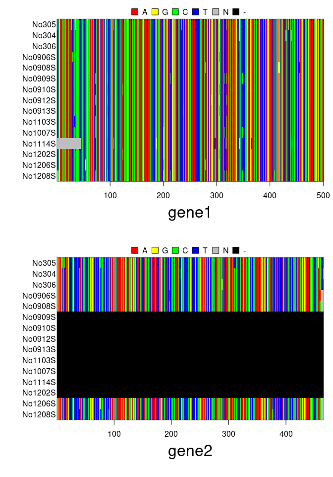
par(oldpar)Like multidna and ape’s DNAbin,
the formal (S4) class multiphyDat is a multi-gene extension
of phangorn’s phyDat class. Data is stored as a
list of phyDat objects, with additional slots for extra
information. The class definition can be obtained by:
getClassDef("multiphyDat")## Class "multiphyDat" [package "apex"]
##
## Slots:
##
## Name: seq type labels n.ind n.seq
## Class: listOrNULL character character integer integer
##
## Name: n.seq.miss ind.info gene.info
## Class: integer data.frameOrNULL data.frameOrNULL
##
## Extends: "multiinfo"phyDat
objects, each corresponding to a given gene/locus, with matching rows
(individuals); unlike multidna which is retrained to DNA
sequences, this class can store any characters, including amino-acid
sequences@dna)Any of these slots can be accessed using @ (see example
below).
As for multidna, multiphyDat objects can be
created via different ways:
new("multiphyDat", ...)multidna object using
multiphyDat2multidnaAs before, we illustrate the use of the constructor below (see
?new.multiphyDat) for more information.
data(Laurasiatherian)
Laurasiatherian
## 47 sequences with 3179 character and 1605 different site patterns.
## The states are a c g t## empty object
new("multiphyDat")## === multiphyDat ===
## [ 0 DNA sequence in 0 gene ]
##
## @type:
## @n.ind: 0 individual
## @n.seq: 0 sequence in total
## @n.seq.miss: 0 gap-only (missing) sequence
## @labels:## simple conversion after artificially splitting data into 2 genes
genes <- list(gene1=Laurasiatherian[,1:1600], gene2=Laurasiatherian[,1601:3179])
x <- new("multiphyDat", genes, type="DNA")
x## === multiphyDat ===
## [ 94 DNA sequences in 2 genes ]
##
## @type: DNA
## @n.ind: 47 individuals
## @n.seq: 94 sequences in total
## @n.seq.miss: 0 gap-only (missing) sequence
## @labels: Platypus Wallaroo Possum Bandicoot Opposum Armadillo...
##
## @seq: (list of phyDat objects)
## $gene1
## 47 sequences with 1600 character and 827 different site patterns.
## The states are a c g t
##
## $gene2
## 47 sequences with 1579 character and 844 different site patterns.
## The states are a c g tSeveral functions facilitate data handling: *
concatenate: concatenate several genes into a single
DNAbin or phyDat matrix *
x[i,j]: subset x by individuals (i) and/or genes (j) *
multidna2multiphyDat: converts from
multidna to multiphyDat *
multiphyDat2multidna: converts from
multiphyDat to multidna
Example code:
files <- dir(system.file(package="apex"),patter="patr", full=TRUE)

## read files
x <- read.multiFASTA(files)
x
## === multidna ===
## [ 32 DNA sequences in 4 genes ]
##
## @n.ind: 8 individuals
## @n.seq: 32 sequences in total
## @n.seq.miss: 8 gap-only (missing) sequences
## @labels: 2340_50156.ab1 2340_50149.ab1 2340_50674.ab1 2370_45312.ab1 2340_50406.ab1 2370_45424.ab1 ...
##
## @dna: (list of DNAbin matrices)
## $patr_poat43
## 8 DNA sequences in binary format stored in a matrix.
##
## All sequences of same length: 764
##
## Labels:
## 2340_50156.ab1
## 2340_50149.ab1
## 2340_50674.ab1
## 2370_45312.ab1
## 2340_50406.ab1
## 2370_45424.ab1
## ...
##
## Base composition:
## a c g t
## 0.320 0.158 0.166 0.356
## (Total: 6.11 kb)
##
## $patr_poat47
## 8 DNA sequences in binary format stored in a matrix.
##
## All sequences of same length: 626
##
## Labels:
## 2340_50156.ab1
## 2340_50149.ab1
## 2340_50674.ab1
## 2370_45312.ab1
## 2340_50406.ab1
## 2370_45424.ab1
## ...
##
## Base composition:
## a c g t
## 0.227 0.252 0.256 0.266
## (Total: 5.01 kb)
##
## $patr_poat48
## 8 DNA sequences in binary format stored in a matrix.
##
## All sequences of same length: 560
##
## Labels:
## 2340_50156.ab1
## 2340_50149.ab1
## 2340_50674.ab1
## 2370_45312.ab1
## 2340_50406.ab1
## 2370_45424.ab1
## ...
##
## Base composition:
## a c g t
## 0.305 0.185 0.182 0.327
## (Total: 4.48 kb)
##
## $patr_poat49
## 8 DNA sequences in binary format stored in a matrix.
##
## All sequences of same length: 556
##
## Labels:
## 2340_50156.ab1
## 2340_50149.ab1
## 2340_50674.ab1
## 2370_45312.ab1
## 2340_50406.ab1
## 2370_45424.ab1
## ...
##
## Base composition:
## a c g t
## 0.344 0.149 0.187 0.320
## (Total: 4.45 kb)oldpar <- par(mar=c(6,11,4,1))
plot(x)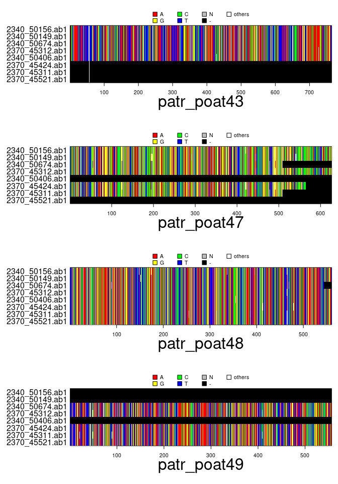
## subset
plot(x[1:3,2:4])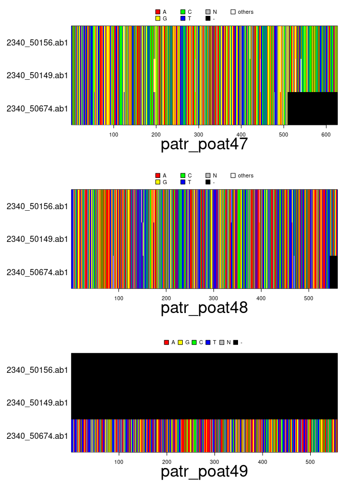
par(oldpar)## concatenate
y <- concatenate(x)
y## 8 DNA sequences in binary format stored in a matrix.
##
## All sequences of same length: 2506
##
## Labels:
## 2340_50156.ab1
## 2340_50149.ab1
## 2340_50674.ab1
## 2370_45312.ab1
## 2340_50406.ab1
## 2370_45424.ab1
## ...
##
## Base composition:
## a c g t
## 0.298 0.187 0.197 0.319
## (Total: 20.05 kb)oldpar <- par(mar=c(5,8,4,1))
image(y)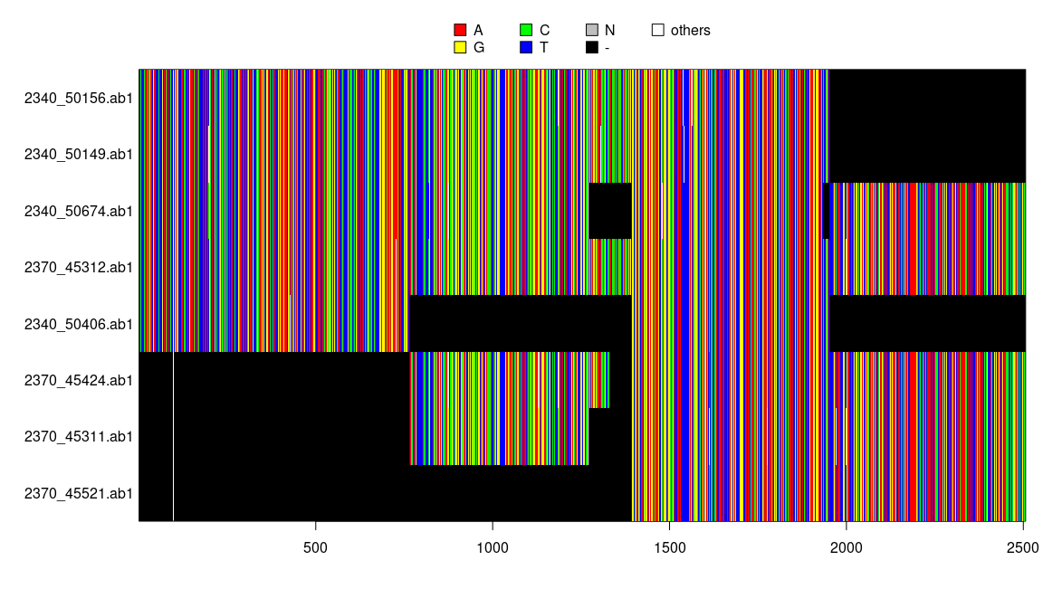
par(oldpar)

## concatenate multiphyDat object
z <- multidna2multiphyDat(x)
u <- concatenate(z)
u
## 8 sequences with 2506 character and 69 different site patterns.
## The states are a c g ttree <- pratchet(u, trace=0, all = FALSE)
oldpar <- par(mar=c(1,1,1,1))
plot(tree, "u")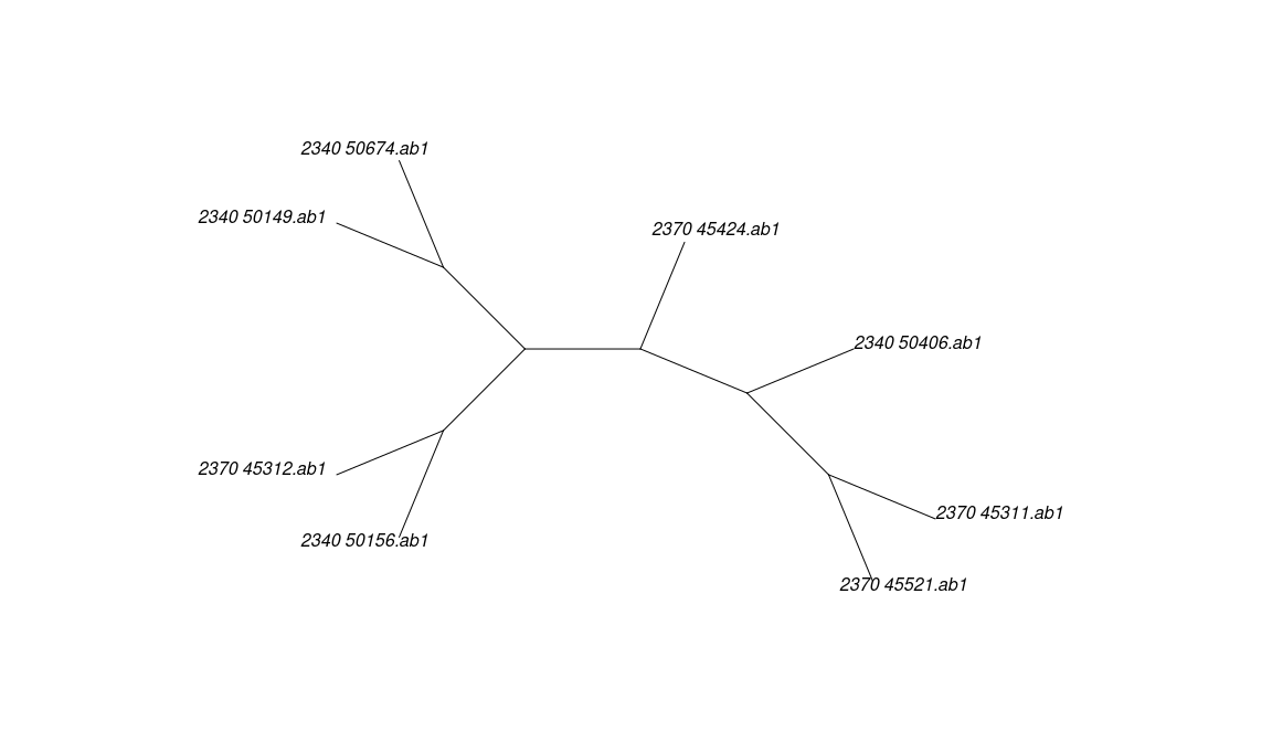
par(oldpar)Distance-based trees (e.g. Neighbor Joining) can be obtained for each
gene in a multidna object using getTree
## make trees, default parameters
trees <- getTree(x)
trees
## 4 phylogenetic treesplot(trees, 4, type="unrooted")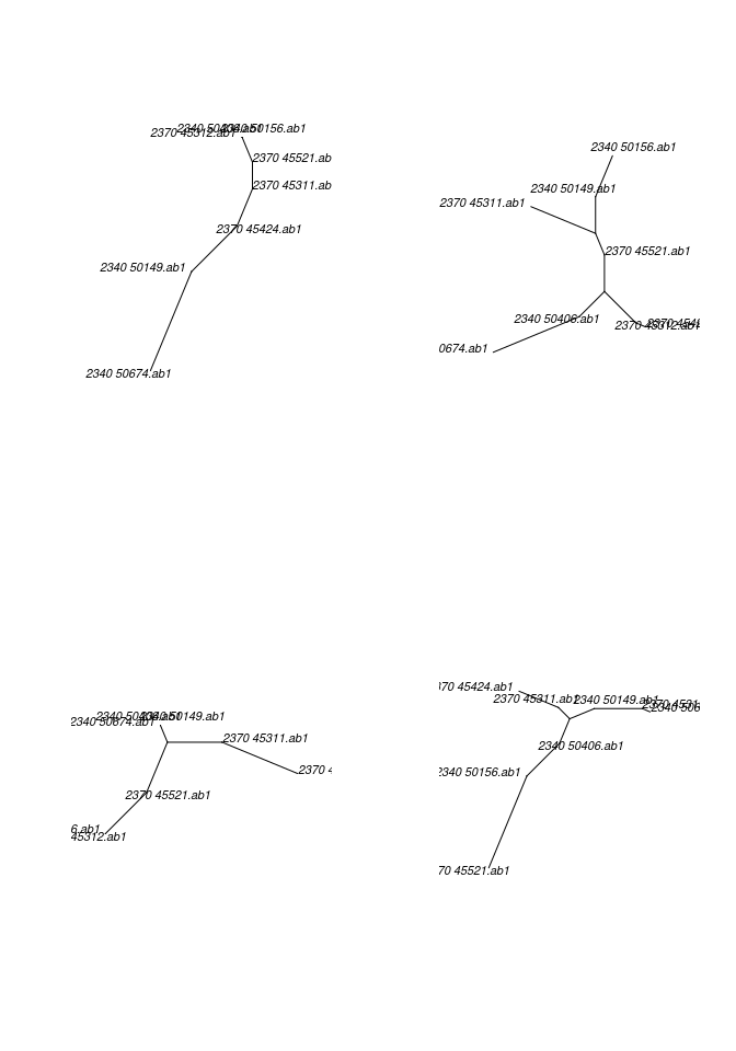
As an alternative, all genes can be pooled into a single alignment to obtain a single tree using:
##
## Phylogenetic tree with 8 tips and 6 internal nodes.
##
## Tip labels:
##   2340_50156.ab1 , 2340_50149.ab1 , 2340_50674.ab1 , 2370_45312.ab1 , 2340_50406.ab1 , 2370_45424.ab1 , ...
##
## Unrooted; includes branch lengths.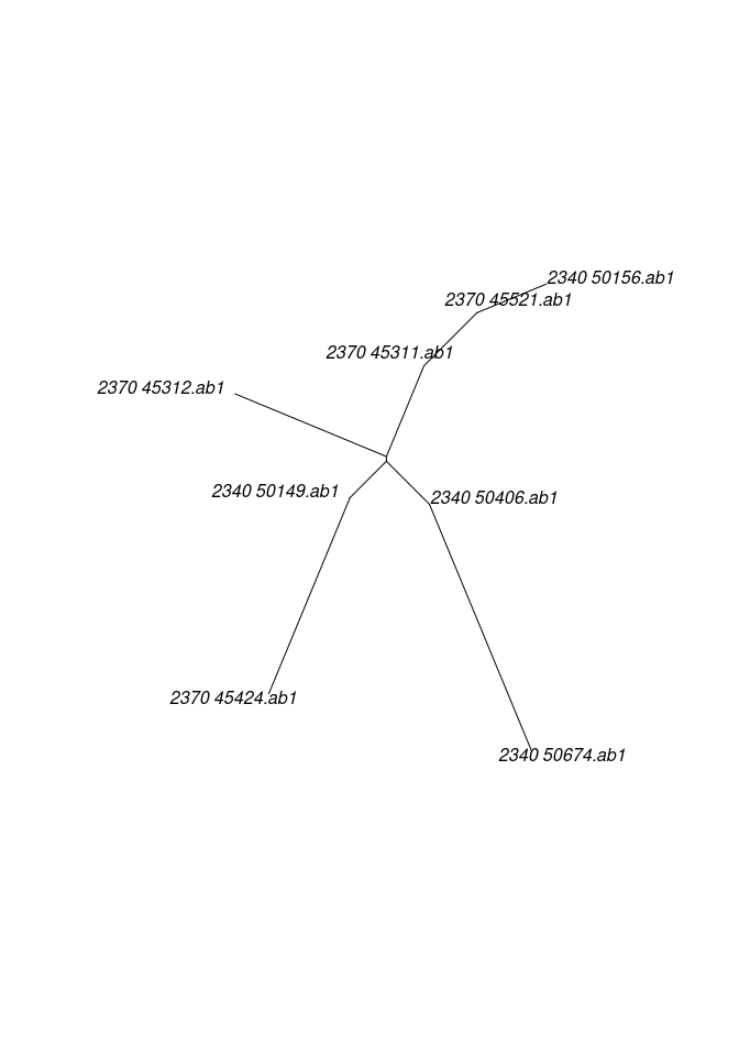
It is also possible to use functions from phangorn to
estimate with maximum likelihood trees. Here is an example using the
multiphyDat object z created in the previous
section:
## input object
z
## build trees
pp <- pmlPart(bf ~ edge + nni, z, control = pml.control(trace = 0))
pp
## convert trees for plotting
trees <- pmlPart2multiPhylo(pp)plot(trees, 4)The following functions enable the export from apex to other
packages: * multidna2genind: concatenates genes and
export SNPs into a genind object; alternatively,
Multi-Locus Sequence Type (MLST) can be used to treat genes as separate
locus and unique sequences as alleles. *
multiphyDat2genind: does the same for multiphyDat
object
This is illustrated below:
## find source files in apex
library(adegenet)
files <- dir(system.file(package="apex"),patter="patr", full=TRUE)

## import data
x <- read.multiFASTA(files)
x
## === multidna ===
## [ 32 DNA sequences in 4 genes ]
##
## @n.ind: 8 individuals
## @n.seq: 32 sequences in total
## @n.seq.miss: 8 gap-only (missing) sequences
## @labels: 2340_50156.ab1 2340_50149.ab1 2340_50674.ab1 2370_45312.ab1 2340_50406.ab1 2370_45424.ab1 ...
##
## @dna: (list of DNAbin matrices)
## $patr_poat43
## 8 DNA sequences in binary format stored in a matrix.
##
## All sequences of same length: 764
##
## Labels:
## 2340_50156.ab1
## 2340_50149.ab1
## 2340_50674.ab1
## 2370_45312.ab1
## 2340_50406.ab1
## 2370_45424.ab1
## ...
##
## Base composition:
## a c g t
## 0.320 0.158 0.166 0.356
## (Total: 6.11 kb)
##
## $patr_poat47
## 8 DNA sequences in binary format stored in a matrix.
##
## All sequences of same length: 626
##
## Labels:
## 2340_50156.ab1
## 2340_50149.ab1
## 2340_50674.ab1
## 2370_45312.ab1
## 2340_50406.ab1
## 2370_45424.ab1
## ...
##
## Base composition:
## a c g t
## 0.227 0.252 0.256 0.266
## (Total: 5.01 kb)
##
## $patr_poat48
## 8 DNA sequences in binary format stored in a matrix.
##
## All sequences of same length: 560
##
## Labels:
## 2340_50156.ab1
## 2340_50149.ab1
## 2340_50674.ab1
## 2370_45312.ab1
## 2340_50406.ab1
## 2370_45424.ab1
## ...
##
## Base composition:
## a c g t
## 0.305 0.185 0.182 0.327
## (Total: 4.48 kb)
##
## $patr_poat49
## 8 DNA sequences in binary format stored in a matrix.
##
## All sequences of same length: 556
##
## Labels:
## 2340_50156.ab1
## 2340_50149.ab1
## 2340_50674.ab1
## 2370_45312.ab1
## 2340_50406.ab1
## 2370_45424.ab1
## ...
##
## Base composition:
## a c g t
## 0.344 0.149 0.187 0.320
## (Total: 4.45 kb)## extract SNPs and export to genind
obj1 <- multidna2genind(x)
obj1## /// GENIND OBJECT /////////
##
## // 8 individuals; 11 loci; 22 alleles; size: 11 Kb
##
## // Basic content
## @tab: 8 x 22 matrix of allele counts
## @loc.n.all: number of alleles per locus (range: 2-2)
## @loc.fac: locus factor for the 22 columns of @tab
## @all.names: list of allele names for each locus
## @ploidy: ploidy of each individual (range: 1-1)
## @type: codom
## @call: DNAbin2genind(x = concatenate(x, genes = genes))
##
## // Optional content
## - empty -The MLST option can be useful for a quick diagnostic of diversity amongst individuals. While it is best suited to clonal organisms, we illustrate this procedure using our toy dataset:
obj3 <- multidna2genind(x, mlst=TRUE)
obj3
## /// GENIND OBJECT /////////
##
## // 8 individuals; 4 loci; 27 alleles; size: 26.8 Kb
##
## // Basic content
## @tab: 8 x 27 matrix of allele counts
## @loc.n.all: number of alleles per locus (range: 6-8)
## @loc.fac: locus factor for the 27 columns of @tab
## @all.names: list of allele names for each locus
## @ploidy: ploidy of each individual (range: 1-1)
## @type: codom
## @call: df2genind(X = xdfnum, ind.names = x@labels, ploidy = 1)
##
## // Optional content
## - empty -## alleles of the first locus (=sequences)
alleles(obj3)[[1]]## [1] "--------------------------------------------------------------------------------------------------------------------------------------------------------------------------------------------------------------------------------------------------------------------------------------------------------------------------------------------------------------------------------------------------------------------------------------------------------------------------------------------------------------------------------------------------------------------------------------------------------------------------------------------------------------------------------------------------------------------------------------------------------------------------------------------"
## [2] "--tacactttgataacaaaaaaatactaatgtaagatgtggttatatttcttgtggctttttatctgatatattgtcttaatgcactatcatactttgatctgaaaagggtctgtgatggaaacctaccacctcttcagttatgcattaaaattacccattataccatcattttgttatataactgaaaagttaatcgtgactttgcaattctggattgctctttctcttgtaaactctttggctttcagaagtcatattaataattttatccttgtttgtgacaaataaatgcatatttaatcttcatgtttaaataatgtgctcttgtaacgtgccaaacaaaaggtgatgaatggtaggggcattttcagtctctcttttagatttccttgtgatgtcagtaaacagaaggagaatttagtctcagtccctagggatgtcttaccattgtaatggaattaagagagctgataaaatgaataattcatgatgtagtatttgttgacaaaacttcttaaaagtccactacagaccagtgaacgtgtggttaggaagtagcaatcattgttccacctcatttttgttgttgtttttccctccattgaactgttgttattaatcataaaataatgaataactgtccttctgtgtcctcccctctaacaaaatataatttaggagggattgtgtagtaaaaccaaacaaaccaaagaagaaacataagaaaagcacaatatatttctcattgaacagagggattt-"
## [3] "--tacactttgataacaaaaaaatactaatgtaagatgtggttatatttcttgtggctttttatctgatatattgtcttaatgcactatcatactttgatctgaaaagggtctgtgatggaaacctaccacctcttcagttatgcattaaaattacccattataccatcattttgttatataactgaaaagttaattgtgactttgcaattctggattgctctttctcttgtaaactctttggctttcagaagtcatattaataattttatccttgtttgtgacaaataaatgcatatttaatcttcatgtttaaataatgtgctcttgtaacgtgccaaacaaaaggtgatgaatggtaggggcattttcagtctctcttttagatttccttgtgatgtcagtaaacagaaggagaatttagtctcagtccctagggatgtcttaccattgtaatggaattaagagagctgataaaatgaataattcatgatgtagtatttgttgacaaaacttcttaaaagtccactacagaccagtgaacgtgtggttaggaagtagcaatcattgttccacctcatttttgttgttgtttttccctccattgaactgttgttattaatcataaaataatgaataactgtccttctgtgtcctcccctctaacaaaatataatttaggagggattgtgtagtaaaaccaaacaaaccaaagaagaaacataagaaaagcacaatatatttctcattgaacagagggattt-"
## [4] "--tacactttgataacaaaaaaatactaatgtaagatgtggttatatttcttgtggctttttatctgatatattgtcttaatgcactatcatactttgatctgaaaagggtctgtgatggaaacctaccacctcttcagttatgcattaaaattacccattataccatcattttgttatataactgaaaagttaattgtgactttgcaattctggattgctctttctcttgtaaactctttggctttcagaagtcatattaataattttatccttgtttgtgacaaataaatgcatatttaatcttcatgtttaaataatgtgctcttgtaacgtgccaaacaaaaggtgatgaatggtaggggcattttcagtctctcttttagatttccttgtgatgtcagtaaacagaaggagaatttagtctcagtccctagggatgtcttaccattgtaatggaattaagagagctgataaaatgaataattcatgatgtagtatttgttgacaaaacttcttaaaagtccactacagaccagtgaacgtgtggttaggaagtagcaatcattgttccacctcatttttgttgttgtttttccctccattgaactgttgttattaatcataaaataatgaataactgtccttctgtgtcctcccctctaacaaaatataatttaggagggattgtgtagtaaaaccaaacaaaccaaagaagaaacataagraaagcacaatatatttctcattgaacagagggattt-"
## [5] "--tacactttgataacaaaaaaatactaatgtaagatgtggttatatttcttgtggctttttatctgatatattgtcttaatgcactatcatactttgatctgaaaagggtctgtgatggaaacctaccacctcttcagttatgcattaaaattacccattataccatcattttgttatataactgaaaagttaattgtgactttgcaattctggattgctctttctcttgtaaactctttggctttcagaagtcatattaataattttatccttgtttgtgacaaataaatgcatatttaatcttcatgtttaaataatgtgctcttgtaacgtgccaaacaaaaggtgatgaatggtaggggcattttcagtctctcttttagatttccttgtgatgtcagtaaacagaaggagaatttagtctcmgtccctagggatgtcttaccattgtaatggaattaagagagctgataaaatgaataattcatgatgtagtatttgttgacaaaacttcttaaaagtccactacagaccagtgaacgtgtggttaggaagtagcaatcattgttccacctcatttttgttgttgtttttccctccattgaactgttgttattaatcataaaataatgaataactgtccttctgtgtcctcccctctaacaaaatataatttaggagggattgtgtagtaaaaccaaacaaaccaaagaagaaacataagraaagcacaatatatttctcattgaacagagggattt-"
## [6] "--tacactttgataacaaaaaaatactaatgtaagatgtggttatatttcttgtggctttttatctgatatattgtcttaatgcactatcatactttgatctgaaaagggtctgtgatggaaacctaccacctcttcagttatgcattaaaattacccattataccatcattttgttatataactgaaaagttaatygtgactttgcaattctggattgctctttctcttgtaaactctttggctttcagaagtcatattaataattttatccttgtttgtgacaaataaatgcatatttaatcttcatgtttaaataatgtgctcttgtaacgtgccaaacaaaaggtgatgaatggtaggggcattttcagtctctcttttagatttccttgtgatgtcagtaaacagaaggagaatttagtctcagtccctagggatgtcttaccattgtaatggaattaagagagctgataaaatgaataattcatgatgtagtatttgttgacaaaacttcttaaaagtccactacagaccagtgaacgtgtggttaggaagtagcaatcattgttccacctcatttttgttgttgtttttccctccattgaactgttgttattaatcataaaataatgaataactgtccttctgtgtcctcccctctaacaaaatataatttaggagggattgtgtagtaaaaccaaacaaaccaaagaagaaacataagaaaagcacaatatatttctcattgaacagagggattt-"