The goal of StempCens is to estimate the parameters of
spatio-temporal models with censored or missing data using the SAEM
algorithm (Delyon, Lavielle, and Moulines 1999). This algorithm is a
stochastic approximation of the widely used EM algorithm and is
particularly useful for models in which the E-step does not have an
analytical form. In addition to providing the expressions used for
parameter estimation in the proposed model, the package includes the
computation of the observed information matrix using the method
developed by Louis (1982). To evaluate the performance of the fitted
model, case-deletion diagnostics are provided (see also Cook 1977; Zhu
et al. 2001). Moreover, the package computes the spatio-temporal
covariance matrix and the effective range for an isotropic spatial
correlation function.
A detailed description of the model can be found in Valeriano et al. (2021).
You can install the released version of StempCens from CRAN with:
install.packages("StempCens")StempCens package provides five functions:
CovarianceM: Computes the spatio-temporal covariance
matrix for balanced data.EffectiveRange: Computes the effective range for an
isotropic spatial correlation function.EstStempCens: Returns the maximum likelihood estimates
of the unknown parameters.PredStempCens: Performs spatio-temporal prediction in a
set of new spatial locations for fixed time points.CrossStempCens: Performs cross-validation, which
measure the performance of the predictive model on new test
dataset.DiagStempCens: Returns measures and graphics for
diagnostic analysis.This is a basic example which shows you how to solve a problem using
functions EstStempCens (parameter estimation) and
PredStempCens (prediction in new locations):
library(StempCens)
set.seed(403020)
# Initial parameter values
beta <- c(-1, 1.50)
phi <- 5
rho <- 0.60
tau2 <- 0.80
sigma2 <- 2
# Simulating data
coord <- matrix(round(runif(100, 0, 10),9), ncol=2)
time <- 1:5
x <- cbind(rexp(250,2), rnorm(250,2,1)) # Covariates
data <- rnStempCens(x, time, coord, beta, phi, rho, tau2,
sigma2, type.S="pow.exp", kappa=0.5,
cens="left", pcens=0.10)
# Splitting the dataset
train <- data[-c(211:220),]
test <- data[211:220,]
sum(test$ci)
#> [1] 0
# Estimation
x <- cbind(train$x1, train$x2)
est_train <- EstStempCens(train$yObs, x, train$ci, train$time, train[,1:2], train$lcl, train$ucl,
init.phi=3.5, init.rho=0.5, init.tau2=1, kappa=0.5, type.S="pow.exp",
IMatrix=TRUE, M=20, perc=0.25, MaxIter=300, pc=0.20)
#>
#> ---------------------------------------------------------------
#> Spatio-temporal models for censored/missing responses
#> ---------------------------------------------------------------
#> Estimates SE
#> β1 -1.1797 0.1877
#> β2 1.6018 0.0910
#> σ² 2.0035 1.4689
#> τ² 0.8095 0.4598
#> ϕ 4.0576 3.7428
#> ρ 0.6035 0.1143
#> The effective range is 36.414 spatial units.
#> --------------------------------------------------------------
#>
#>
#> Model selection criteria
#> ------------------------------------
#> Value
#> Loglik. -384.689
#> AIC 781.377
#> AICcorr. 781.738
#> BIC 802.261
#> ------------------------------------
#>
# Prediction
xPre <- cbind(test$x1, test$x2)
pre_teste <- PredStempCens(est_train, test[,1:2], test$time, xPre)
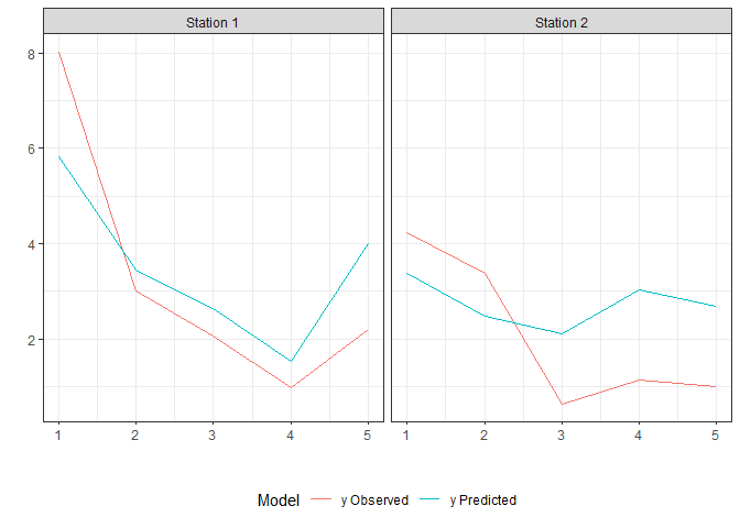
library(ggplot2)
Model <- rep(c("y Observed","y Predicted"),each=10)
station <- rep(rep(c("Station 1", "Station 2"),each=5), times=2)
xcoord1 <- rep(seq(1:5),4)
ycoord1 <- c(test$yObs, pre_teste$predValues)
data2 <- data.frame(Model,station,xcoord1,ycoord1)
ggplot(data=data2, aes(x=xcoord1, y=ycoord1)) + geom_line(aes(color=Model)) + theme_bw() +
facet_wrap(station~.,nrow=1) + labs(x="",y="") + theme(legend.position="bottom")
For diagnostic analysis, the input parameter IMatrix
needs to be TRUE in the EstStempCens
function.
diag <- DiagStempCens(est_train, type.diag="location", diag.plot = TRUE, ck=1)